Download
1 / 8
80 likes | 326 Views
Bertrand Again. Here we study a situation known as capacity constraints. Say the demand in the market is Q = 6000-60P. Say we have two firms who will compete on price as in the Bertrand duopoly situation and each has a constant marginal cost = 10.

E N D
Bertrand Again Here we study a situation known as capacity constraints.
Say the demand in the market is Q = 6000-60P. Say we have two firms who will compete on price as in the Bertrand duopoly situation and each has a constant marginal cost = 10. Let’s see what the result would be if there was only one firm in this market. With Q = 6000 - 60P P = 6000/60 – (1/60)Q MR = 6000/60 – (2/60)Q and with MR = MC for profit maximization 6000/60 – (2/60)Q = 10, so Q = (6000-600)/2 = 2700 and then P = 55. Next, let’s look at the best price response for each firm in a Bertrand duopoly situation.
Firm 2’s best price response If P1 > monopoly price of 55, set P2 = 55 and sell monopoly Q, 10(=mc) < P1 <= 55, set P2 = P1 – small amount, sell all of mkt at P2, P1 = 10(=mc), set P2 = 10(=mc) and sell half of market at P2 = 10, 10(=mc) > P1 >= 0, set P2 > P1 and sell nothing. Firm 1’s best price response is similar If P2 > monopoly price of 55, set P1 = 55 and sell monopoly Q, 10(=mc) < P2<= 55, set P1 = P2 – small amount, sell all of mkt at P1, P2 = 10(=mc), set P1= 10(=mc) and sell half of market at P1 = 10, 10(=mc) > P2 >= 0, set P1 > P2 and sell nothing.
Now, although we really haven’t mentioned it explicitly, both firms recognize each other’s best price response. So, each recognizes what are the options for the other. For example, firm 2 recognizes that firm 1 has a best price response. Plus firm 2 believes as a credible position that firm 1 will want to have a lower price than firm 2’s if firm 2 makes the price, say, 45 in our example. In the context of the economic literature, it is said that firm 1 threatens to lower the price if firm 2 makes its price 45, and firm 2 sees it as a credible threat. Firm 1 see similar credible threats. Economic actors must deal with credible threats.
So, we haven’t done anything new here yet except introduce the notion of credible threats. We just looked at a new problem. The Nash equilibrium price for each will be 10 and in the market Q will be 5400. Each will take half of 5400, for a Q of 2700 for each. Up to this point we have assumed that each firm had the capacity to meet the demand. But, let’s now say that firm 1 can only make 1000 units and firm 2 can only make 1400. When you look at the market demand, 2400 units could be sold at a price of : 2400 = 6000 – 60P, or P = (6000 – 2400)/60 = 60. How does each firm view each others best price response in the context of capacity constraints?
Here is a new wrinkle in firm 2’s thinking. If I, firm 2, put a price of 60 on the product, then from firm 1’s best price response function I see firm 1 will set a price of 55. But I do not view it as credible because at a price of 55 it will have too much demand. In other words, if you can charge 1000 people 60 because they will pay it, why charge them 55? So, in the face of capacity constraints firm 2 does not see firm 1’s best price response function as credible. Firm 1 has a similar view of firm 2’s best price response function. The authors suggest that in the face of capacity constraints the Bertrand duopoly model does not result in the competitive solution. Next, let’s look at how the authors add to the discussion by considering residual demand curves.
The total demand we saw before was Q = 6000 – 60P. If P = 60 the Q = 2400 and the firms could each get their capacity amount. Another way to see things from firm 2’s perspective: If firm 1 makes P = 60 and takes 1000 customers, then my residual demand will be Q = 6000 – 1000 – 60P = 5000 – 60P and if I, firm 2, make P=60 I will have Q = 5000 – 3600 = 1400, my capacity constraint. Let’s see if firm 2 can do better by taking the residual demand and act like a monopolist with that demand. With Q = 5000 – 60P, P = 5000/60 – (1/60)Q and MR = 5000/60 – (2/60)Q. Then with MR = MC, the best Q in a perfect world with no capacity problems would be
5000/60 – (2/60)Q = 10, so Q = (5000 – 600)/2 = 2200 and the price would be (5000 – 2200)/60 = 46.67. So, firm 2 says, hey, if firm 1 does a price of 60 I might as well do 60 as well because if I try a price of 46.67 I would attract 2200 but can only serve 1400 so I might as well charge those 1400 peopel 60 instead of 46.67. Firm 1 will similarly see its residual demand if firm 2 has P = 60 as Q = 6000 – 1400 – 60P. Thus P = 4600/60 – (1/60)Q and MR = 4600/60 – (2/60)Q and with MR = MC Q = (4600 – 600)/2 = 2000 and P = (4600 – 2000)/60 = 43.33. Firm 1 will say why charge 2000 people 43.33 when I can only serve 1000 of them. Just charge the 1000 people the 60. In the face of capacity constraints in Bertrand model the competitive solution will not result because it is not a credible solution.