Download
1 / 84
860 likes | 1k Views
CSG230 Summary. Donghui Zhang. What we learned?. Frequent pattern & association Clustering Classification Data warehousing Additional. What we learned?. Frequent pattern & association frequent itemsets (Apriori, FP-growth) max and closed itemsets association rules essential rules

E N D
CSG230 Summary Donghui Zhang Data Mining: Concepts and Techniques
What we learned? • Frequent pattern & association • Clustering • Classification • Data warehousing • Additional Data Mining: Concepts and Techniques
What we learned? • Frequent pattern & association • frequent itemsets (Apriori, FP-growth) • max and closed itemsets • association rules • essential rules • generalized itemsets • Sequential pattern • Clustering • Classification • Data warehousing • Additional Data Mining: Concepts and Techniques
What we learned? • Frequent pattern & association • Clustering • k-means • Birch (based on CF-tree) • DBSCAN • CURE • Classification • Data warehousing • Additional Data Mining: Concepts and Techniques
What we learned? • Frequent pattern & association • Clustering • Classification • decision tree • naïve Baysian classifier • Baysian network • neural net and SVM • Data warehousing • Additional Data Mining: Concepts and Techniques
What we learned? • Frequent pattern & association • Clustering • Classification • Data warehousing • concept, schema • data cube & operations (rollup, …) • cube computation: multi-way array aggregation • iceberg cube • dynamic data cube • Additional Data Mining: Concepts and Techniques
What we learned? • Frequent pattern & association • Clustering • Classification • Data warehousing • Additional • lattice (of itemsets, g-itemsets, rules, cuboids) • distance-based indexing Data Mining: Concepts and Techniques
Frequent pattern & association • frequent itemsets (Apriori, FP-growth) • max and closed itemsets • association rules • essential rules • generalized itemsets • Sequential pattern Data Mining: Concepts and Techniques
Customer buys both Customer buys diaper Customer buys beer Basic Concepts: Frequent Patterns and Association Rules • Itemset X={x1, …, xk} • Find all the rules XYwith min confidence and support • support, s, probability that a transaction contains XY • confidence, c,conditional probability that a transaction having X also contains Y. • Let min_support = 50%, min_conf = 50%: • A C (50%, 66.7%) • C A (50%, 100%) Data Mining: Concepts and Techniques
From Mining Association Rules to Mining Frequent Patterns (i.e. Frequent Itemsets) • Given a frequent itemset X, how to find association rules? • Examine every subset S of X. • Confidence(SX – S ) = support(X)/support(S) • Compare with min_conf • An optimization is possible (refer to exercises 6.1, 6.2). Data Mining: Concepts and Techniques
The Apriori Algorithm—An Example Database TDB L1 C1 1st scan C2 C2 L2 2nd scan L3 C3 3rd scan Data Mining: Concepts and Techniques
Important Details of Apriori • How to generate candidates? • Step 1: self-joining Lk • Step 2: pruning • How to count supports of candidates? • Example of Candidate-generation • L3={abc, abd, acd, ace, bcd} • Self-joining: L3*L3 • abcd from abc and abd • acde from acd and ace • Pruning: • acde is removed because ade is not in L3 • C4={abcd} Data Mining: Concepts and Techniques
Construct FP-tree from a Transaction Database TID Items bought (ordered) frequent items 100 {f, a, c, d, g, i, m, p}{f, c, a, m, p} 200 {a, b, c, f, l, m, o}{f, c, a, b, m} 300 {b, f, h, j, o, w}{f, b} 400 {b, c, k, s, p}{c, b, p} 500{a, f, c, e, l, p, m, n}{f, c, a, m, p} min_support = 3 Header Table Item frequency head f 4 c 4 a 3 b 3 m 3 p 3 • Scan DB once, find frequent 1-itemset (single item pattern) • Sort frequent items in frequency descending order, f-list • Scan DB again, construct FP-tree F-list=f-c-a-b-m-p Data Mining: Concepts and Techniques
Construct FP-tree from a Transaction Database TID Items bought (ordered) frequent items 100 {f, a, c, d, g, i, m, p}{f, c, a, m, p} 200 {a, b, c, f, l, m, o}{f, c, a, b, m} 300 {b, f, h, j, o, w}{f, b} 400 {b, c, k, s, p}{c, b, p} 500{a, f, c, e, l, p, m, n}{f, c, a, m, p} min_support = 3 {} Header Table Item frequency head f 4 c 4 a 3 b 3 m 3 p 3 • Scan DB once, find frequent 1-itemset (single item pattern) • Sort frequent items in frequency descending order, f-list • Scan DB again, construct FP-tree f:1 c:1 a:1 m:1 F-list=f-c-a-b-m-p p:1 Data Mining: Concepts and Techniques
Construct FP-tree from a Transaction Database TID Items bought (ordered) frequent items 100 {f, a, c, d, g, i, m, p}{f, c, a, m, p} 200 {a, b, c, f, l, m, o}{f, c, a, b, m} 300 {b, f, h, j, o, w}{f, b} 400 {b, c, k, s, p}{c, b, p} 500{a, f, c, e, l, p, m, n}{f, c, a, m, p} min_support = 3 {} Header Table Item frequency head f 4 c 4 a 3 b 3 m 3 p 3 • Scan DB once, find frequent 1-itemset (single item pattern) • Sort frequent items in frequency descending order, f-list • Scan DB again, construct FP-tree f:2 c:2 a:2 m:1 b:1 F-list=f-c-a-b-m-p p:1 m:1 Data Mining: Concepts and Techniques
Construct FP-tree from a Transaction Database TID Items bought (ordered) frequent items 100 {f, a, c, d, g, i, m, p}{f, c, a, m, p} 200 {a, b, c, f, l, m, o}{f, c, a, b, m} 300 {b, f, h, j, o, w}{f, b} 400 {b, c, k, s, p}{c, b, p} 500{a, f, c, e, l, p, m, n}{f, c, a, m, p} min_support = 3 {} Header Table Item frequency head f 4 c 4 a 3 b 3 m 3 p 3 • Scan DB once, find frequent 1-itemset (single item pattern) • Sort frequent items in frequency descending order, f-list • Scan DB again, construct FP-tree f:3 c:2 b:1 a:2 m:1 b:1 F-list=f-c-a-b-m-p p:1 m:1 Data Mining: Concepts and Techniques
Construct FP-tree from a Transaction Database TID Items bought (ordered) frequent items 100 {f, a, c, d, g, i, m, p}{f, c, a, m, p} 200 {a, b, c, f, l, m, o}{f, c, a, b, m} 300 {b, f, h, j, o, w}{f, b} 400 {b, c, k, s, p}{c, b, p} 500{a, f, c, e, l, p, m, n}{f, c, a, m, p} min_support = 3 {} Header Table Item frequency head f 4 c 4 a 3 b 3 m 3 p 3 • Scan DB once, find frequent 1-itemset (single item pattern) • Sort frequent items in frequency descending order, f-list • Scan DB again, construct FP-tree f:3 c:1 c:2 b:1 b:1 a:2 p:1 m:1 b:1 F-list=f-c-a-b-m-p p:1 m:1 Data Mining: Concepts and Techniques
Construct FP-tree from a Transaction Database TID Items bought (ordered) frequent items 100 {f, a, c, d, g, i, m, p}{f, c, a, m, p} 200 {a, b, c, f, l, m, o}{f, c, a, b, m} 300 {b, f, h, j, o, w}{f, b} 400 {b, c, k, s, p}{c, b, p} 500{a, f, c, e, l, p, m, n}{f, c, a, m, p} min_support = 3 {} Header Table Item frequency head f 4 c 4 a 3 b 3 m 3 p 3 • Scan DB once, find frequent 1-itemset (single item pattern) • Sort frequent items in frequency descending order, f-list • Scan DB again, construct FP-tree f:4 c:1 c:3 b:1 b:1 a:3 p:1 m:2 b:1 F-list=f-c-a-b-m-p p:2 m:1 Data Mining: Concepts and Techniques
{} Header Table Item frequency head f 4 c 4 a 3 b 3 m 3 p 3 f:4 c:1 c:3 b:1 b:1 a:3 p:1 m:2 b:1 p:2 m:1 Find Patterns Having P From P-conditional Database • Starting at the frequent item header table in the FP-tree • Traverse the FP-tree by following the link of each frequent item p • Accumulate all of transformed prefix paths of item p to form p’s conditional pattern base Conditional pattern bases item cond. pattern base c f:3 a fc:3 b fca:1, f:1, c:1 m fca:2, fcab:1 p fcam:2, cb:1 Data Mining: Concepts and Techniques
Max-patterns • Frequent pattern {a1, …, a100} (1001) + (1002) + … + (110000) = 2100-1 = 1.27*1030 frequent sub-patterns! • Max-pattern: frequent patterns without proper frequent super pattern • BCDE, ACD are max-patterns • BCD is not a max-pattern Min_sup=2 Data Mining: Concepts and Techniques
B (CDE) C (DE) D (E) E () A (BCDE) Example (ABCDEF) Min_sup=2 Max patterns: Data Mining: Concepts and Techniques
(ABCDEF) Example B (CDE) C (DE) D (E) E () A (BCDE) Min_sup=2 Node A Max patterns: Data Mining: Concepts and Techniques
(ABCDEF) Example B (CDE) C (DE) D (E) E () A (BCDE) Min_sup=2 Node A Max patterns: Data Mining: Concepts and Techniques
(ABCDEF) Example B (CDE) C (DE) D (E) E () A (BCDE) Min_sup=2 Node B Max patterns: Data Mining: Concepts and Techniques
(ABCDEF) Example B (CDE) C (DE) D (E) E () A (BCDE) Min_sup=2 Node B Max patterns: Data Mining: Concepts and Techniques
(ABCDEF) Example B (CDE) C (DE) D (E) E () A (BCDE) Min_sup=2 Max patterns: Data Mining: Concepts and Techniques
A Critical Observation • A→BC has smaller support and confidence than the other rules, independent to the TDB. • Rules AB → C, AC→ B, A→ B and A→ C are redundant with regard to A → BC. • While mining association rules, a large percentage of rules may be redundant. Data Mining: Concepts and Techniques
Formal Definition of Essential Rule • Definition 1Rule r1implies another rule r2 if support(r1)≤support(r2) and confidence(r1)≤ confidence(r2) independent to TDB. • Denote as r1 r2 • Definition 2Rule r1 is an essential rule if r1 is strong and r2 s.t. r2 r1 . Data Mining: Concepts and Techniques
Example of a Lattice of rules ABC CAB BAC ABC AC AB ABC ACB BC BA BCA CB CA • Generate the child nodes: move or delete from the consequent. • To find essential rules: start from each max itemset; browse top-down; prune a sub-tree whenever a rule is confident. Data Mining: Concepts and Techniques
Frequent generalized itemsets • A taxonomy of items. • TDB involves leaf items in the taxonomy. • A g-itemset may contain g-items, but cannot contain an ancestor and a descendant at the same time. • !! A descendant g-item is a “superset”!! • Anyone who bought {milk, bread} also bought {milk}. • Anyone who bought {A} also bought {W}. • ?? how to find frequent g-itemsets? • Browse (and prune) a lattice of g-itemsets! • To get children, replace one item by its ancestor (if conflicts, remove instead.) Data Mining: Concepts and Techniques
What Is Sequential Pattern Mining? • Given a set of sequences, find the complete set of frequent subsequences A sequence database Given support thresholdmin_sup =2, <(ab)c> is a sequential pattern Data Mining: Concepts and Techniques
Mining Sequential Patterns by Prefix Projections • Step 1: find length-1 sequential patterns • <a>, <b>, <c>, <d>, <e>, <f> • Step 2: divide search space. The complete set of seq. pat. can be partitioned into 6 subsets: • The ones having prefix <a>; • The ones having prefix <b>; • … • The ones having prefix <f> Data Mining: Concepts and Techniques
Finding Seq. Patterns with Prefix <a> • Only need to consider projections w.r.t. <a> • <a>-projected database: <(abc)(ac)d(cf)>, <(_d)c(bc)(ae)>, <(_b)(df)cb>, <(_f)cbc> • Find all the length-2 seq. pat. Having prefix <a>: <aa>, <ab>, <(ab)>, <ac>, <ad>, <af>, by checking the frequency of items like a and _a. • Further partition into 6 subsets • Having prefix <aa>; • … • Having prefix <af> Data Mining: Concepts and Techniques
2. Clustering • k-means • Birch (based on CF-tree) • DBSCAN • CURE Data Mining: Concepts and Techniques
The K-Means Clustering Method • Pick k objects as initial seed points • Assign each object to the cluster with the nearest seed point • Re-compute each seed point as the centroid (or mean point) of its cluster • Go back to Step 2, stop when no more new assignment Not optimal. A counter example? Data Mining: Concepts and Techniques
BIRCH (1996) Balanced Iterative Reducing and Clustering using Hierarchies • Birch: Balanced Iterative Reducing and Clustering using Hierarchies, by Zhang, Ramakrishnan, Livny (SIGMOD’96) • Incrementally construct a CF (Clustering Feature) tree, a hierarchical data structure for multiphase clustering • Phase 1: scan DB to build an initial in-memory CF tree (a multi-level compression of the data that tries to preserve the inherent clustering structure of the data) • Phase 2: use an arbitrary clustering algorithm to cluster the leaf nodes of the CF-tree • Scales linearly: finds a good clustering with a single scan and improves the quality with a few additional scans • Weakness: handles only numeric data, and sensitive to the order of the data record. Data Mining: Concepts and Techniques
Clustering Feature Vector Clustering Feature:CF = (N, LS, SS) N: Number of data points LS: Ni=1 Xi SS: Ni=1 (Xi )2 CF = (5, (16,30),244) (3,4) (2,6) (4,5) (4,7) (3,8) Data Mining: Concepts and Techniques
Some Characteristics of CF • Two CF can be aggregated. • Given CF1=(N1, LS1, SS1), CF2 = (N2, LS2, SS2), • If combined into one cluster, CF=(N1+N2, LS1+LS2, SS1+SS2). • The centroid and radius can both be computed from CF. • centroid is the center of the cluster • radius is the average distance between an object and the centroid. • how? Data Mining: Concepts and Techniques
Some Characteristics of CF Data Mining: Concepts and Techniques
CF-Tree in BIRCH • Clustering feature: • summary of the statistics for a given subcluster: the 0-th, 1st and 2nd moments of the subcluster from the statistical point of view. • registers crucial measurements for computing cluster and utilizes storage efficiently • A CF tree is a height-balanced tree that stores the clustering features for a hierarchical clustering • A nonleaf node in a tree has descendants or “children” • The nonleaf nodes store sums of the CFs of their children • A CF tree has two parameters • Branching factor: specify the maximum number of children. • threshold T: max radius of sub-clusters stored at the leaf nodes Data Mining: Concepts and Techniques
Insertion in a CF-Tree • To insert an object o to a CF-tree, insert to the root node of the CF-tree. • To insert o into an index node, insert into the child node whose centroid is the closest to o. • To insert o into a leaf node, • If an existing leaf entry can “absorb” it (i.e. new radius <= T), let it be; • Otherwise, create a new leaf entry. • Split: • Choose two entries whose centroids are the farthest away; • Assign them to two different groups; • Assign the remaining entries to one of these groups. Data Mining: Concepts and Techniques
Density-Based Clustering: Background (II) • Density-reachable: • A point p is density-reachable from a point q wrt. Eps, MinPts if there is a chain of points p1, …, pn, p1 = q, pn = p such that pi+1 is directly density-reachable from pi • Density-connected • A point p is density-connected to a point q wrt. Eps, MinPts if there is a point o such that both, p and q are density-reachable from o wrt. Eps and MinPts. p p1 q p q o Data Mining: Concepts and Techniques
Outlier Border Eps = 1cm MinPts = 5 Core DBSCAN: Density Based Spatial Clustering of Applications with Noise • Relies on a density-based notion of cluster: A cluster is defined as a maximal set of density-connected points • Discovers clusters of arbitrary shape in spatial databases with noise Data Mining: Concepts and Techniques
DBSCAN: The Algorithm • Arbitrary select a point p • Retrieve all points density-reachable from p wrt Eps and MinPts. • If p is a core point, a cluster is formed. • If p is a border point, no points are density-reachable from p and DBSCAN visits the next point of the database. • Continue the process until all of the points have been processed. Data Mining: Concepts and Techniques
Motivation for CURE • k-means does not perform well on this; • AGNES + dmin has single-link effect! Data Mining: Concepts and Techniques
Cure: The Basic Version • Initially, insert to PQ every object as a cluster. • Every cluster in PQ has: • (Up to) C representative points • Pointer to closest cluster (dist between two clusters = min{dist(rep1, rep2)}. • While PQ has more than k clusters, Merge the top cluster with its closest cluster. Data Mining: Concepts and Techniques
Representative points • Step 1: choose up to C points. • If a cluster has no more than C points, all of them. • Otherwise, choose the first point as the farthest from the mean. Choose the others as the farthest from the chosen ones. • Step 2: shrink each point towards mean: • p’ = p + * (mean – p) • [0,1]. Larger means shrinking more. • Reason for shrink: avoid outlier, as faraway objects are shrunk more. Data Mining: Concepts and Techniques
3. Classification • decision tree • naïve Baysian classifier • Baysian net • neural net and SVM Data Mining: Concepts and Techniques
Training Dataset This follows an example from Quinlan’s ID3 Data Mining: Concepts and Techniques
Output: A Decision Tree for “buys_computer” age? <=30 overcast >40 30..40 student? credit rating? yes no yes fair excellent no yes no yes Data Mining: Concepts and Techniques