s implified methods for electronic structure calculations

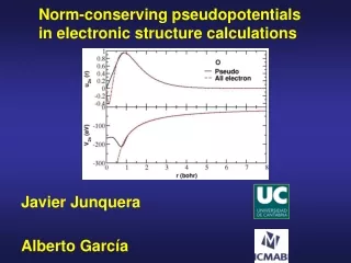
1. simplified methods for electronic structure calculations Jorge Kohanoff Queen’s University Belfast United Kingdom j.kohanoff@qub.ac.uk CCMS Summer Institute LLNL 23 July 2012

2. Queen’s University BelfastNorthern Ireland, UK

3. the problem: nuclei and electrons interacting via Coulomb forces • Hamiltonian of the universe • Schrödinger equation: • r={ri } i=1,...,N • R={RI } I=1,...,P

4. Computational methods 100 1000 10000 100000 1000000 High QM/MM Orbital-free DFT Classical Force fields Accuracy Semi-empirical Tight-binding Ab initio DFT Low Size (number of atoms)

5. Computational methods 100 1000 10000 100000 1000000 High Accuracy Ab initio DFT Low Size (number of atoms)

6. Chemistry vs physics or …when physics meets chemistry? Quantum Chemistry Postulate an approximate many-electron wave function and find it by minimizing the expectation value of the energy for this wave function (Rayleigh-Ritz variational principle). Wave function (ab initio) methods Condensed Matter Physics Express the energy of the system as an approximate functional of the electronic density. This functional is minimized with respect to the density, subject to a normalization constraint. Density functional (first principles) methods

7. Simplified electronic structure methods: general principles (Pople and Beveridge) • Treating electrons explicitly is expensive. • No electrons at all is generally insufficient. • The method should be sufficiently simple to allow for the study of large systems • Approximations shouldn’t modify significantly the physical and chemical properties of the system, e.g. structure, energy levels, vibrations, etc. • The approximate wave function should be as unbiased as possible • Method should take into account active (valence) electrons • It should be sufficiently general to allow for systematic improvements. Ideally, it should be possible to derive it from ab initio through controlled approximations.

8. Computational methods 100 1000 10000 100000 1000000 High QM/MM Orbital-free DFT Classical Force fields Accuracy Semi-empirical Tight-binding Ab initio DFT Low Size (number of atoms)

9. Computational methods 100 1000 10000 100000 1000000 High Classical Force fields Accuracy Low Size (number of atoms)

10. Empirical (classical) force fields • Many-body expansion (2-, 3-, 4-body): general purpose FF, have been tuned mostly for biological systems (AMBER, CHARMM, GROMACS, LAMMPS). Can be used for other systems, but generally require validation and re-calibration (e.g. ionic liquids). • Embedded atom models (many-body): useful for systems with delocalized electrons like metals (Al, Au, Ni). The electronic information is included in the embedding many-body potential. BOPs. • Polarizable and Shell models: Developed to introduce oxygen (electronic) polarization in oxides (e.g. ferroelectric perovskites). They introduce either point dipoles or an electronic shell variable that can displace with respect to the core, thus generating a dipole. Dipoles/shells have to be adjusted self-consistently. • Reactive force fields: Useful to describe systems where there are specific chemical changes (reactions). Extremely efficient, but generally ad hoc for a particular system. • Combining systems is not obvious, e.g. metals with water or oxides

11. Computational methods 100 1000 10000 100000 1000000 High QM/MM Orbital-free DFT Classical Force fields Accuracy Semi-empirical Tight-binding Ab initio DFT Low Size (number of atoms)

12. Computational methods 100 1000 10000 100000 1000000 High Orbital-free DFT Accuracy Low Size (number of atoms)

13. orbital-free or density-only functional methods • Thomas-Fermi (1927): Approximation for the kinetic energy from the homogeneous electron gas. • Minimizing the functional with respect to (r), under the constraint that (r) integrates to N, we obtain an integral equation for (r):  = electronic chemical potential Dirac exchange Wigner correlation Von Weiszäcker gradient correction to T Functional minimization

14. orbital-free or density-only functional methods • Based on Thomas-Fermi idea, these methods require solving a single integro-differential equation. • Need kinetic energy as explicit functional of the density. It’s an unsolved problem. Otherwise, we would all be using OF-DFT. • Inspired in the homogeneous electron gas, they tend to work quite well for simple metals: Na, K (alkaline). • For “less-simple” (sp) metals, e.g. Al, the TF-vW kinetic functional is not good enough. Non-local versions that impose linear response improves a lot (Smargiassi and Madden 1994, Wang et al, 1999).

15. orbital-free or density-only functional methods • TTF does not reproduce the shell structure for atoms. This can be introduced by an ad hoc modulating function (r) in the kinetic functional (King and Handy, 2001) • Also non-local linear response functionals help with the shell structure. • OF-DFT admits only local external potentials. • Core-electrons can be removed by introducing pseudopotentials, but these must be local, which is possible but not easy (Carter).

16. Computational methods 100 1000 10000 100000 1000000 High QM/MM Orbital-free DFT Classical Force fields Accuracy Semi-empirical Tight-binding Ab initio DFT Low Size (number of atoms)

17. Computational methods 100 1000 10000 100000 1000000 High QM/MM Accuracy Low Size (number of atoms)

18. QM/MM • Treat relevant part of the system quantum-mechanically (QM), and the rest classically (MM). • Chemical reactions in a solvent • Active site of enzymes • Two main cases • No chemical bonds between QM and MM • QM and MM regions involve chemical bonds • Part of the system can be treated as a polarizable continuum, or reaction field (RF) • Energy: Q, R,

19. QM/MM • QM-MM interaction energy: • Hamiltonian: QM wfn feels the electrostatics from MM region • Forces: • QM nuclei feel electrostatics and SR repulsion from MM particles • MM particles feel electrostatics from nuclei and electrons + SR repulsion Short-range replusion Avoids Q<0 collapsing onto QM nuclei Electrostatics: e-n + n-n

20. QM/MM • Cutting chemical bonds: electrons in the QM region must “believe” that on the MM side there are orbitals to make bonds. • The safest strategy is to cut homoatomic bonds, e.g. C-C, and replace the MM part with a pseudopotential(Laio) or frozen orbitals (Monard) • MM force fields should be compatible with the QM model • Reaction field: mimics the dielectric response of the medium. • Onsager: QM dipole moment polarizes the medium, which in return produces an electric field back in QM: • Over-polarization (catastrophe) • Improvements: PCM, Oniom, etc. C C MM O N QM

21. Computational methods 100 1000 10000 100000 1000000 High QM/MM Orbital-free DFT Classical Force fields Accuracy Semi-empirical Tight-binding Ab initio DFT Low Size (number of atoms)

22. Computational methods 100 1000 10000 100000 1000000 High Accuracy Semi-empirical Tight-binding Low Size (number of atoms)

23. solving ks/hf equations • Kohn-Sham equations: • to be solved self-consistently (Hartree-Fock similar) -------------------------------------------------------------------------------------------------------------------------------------------------------------------------------------------------------------------------- Nuclear-electron interactionBasis sets All-electron Basis functions (), Size (M) Pseudopotentials Density constructed with KS orbitals fn = occupation numbers KS/HF orbitals must be orthogonal

24. basis sets • Basis set representation of one-electron orbitals: • (r) can depend on energy (eigenvalue). In that case one has to solve a complex non-linear secular equation (e.g. KKR) • If they are energy-independent, the KS equations become a Generalized Eigenvalue Problem: • The same can be done for Hartree-Fock (Roothaan-Hall eq.) (r) = Basis functions Expansion coefficients Hamiltonian Overlap

25. local orbitals • Atom-centered basis functions: • Types: • Atomic orbitals (AO) • Slater-type orbitals (STO): exp(- r) • Gaussian-type orbitals (GTO): exp(- r2) • Numerical • Generally these are non-orthogonal • Löwdinorthogonalization: • Standard Eigenvalue Problem: RI = atomic positions (can use other positions)

26. the hamiltonian in a local basis • One-electron orbitals: • M = number of basis functions • P = number of atoms • Eigenvalue equation: • Overlap matrix: • Size of basis set (M) • SZ: One function per occupied orbital (in the neutral atom) • DZ: Two functions per occupied orbital • DZP: Two functions per occupied orbital and one per empty orbital • Example: O(1s22s22p4). SZ: 1s+3p / DZ: 2s+6p / DZP: 2s+6p+5d

27. the density matrix • Differential overlaps: • Electronic density: • Density matrix: Two-point density (r,r’) expressed in a local basis. • Bond orders: Strength of the bond between two atoms IJ ss s s

28. The hamiltonian matrix • Fock matrix: • KS matrix: • One-electron operator: • Kinetic integrals: • Nuclear attraction: • I=J=K: One-center integrals • IJ=K: Two-center integrals (and permutations) • IJK: Three-centerintegrals

29. Total energy and density matrix • Two-electron integrals (Coulomb and Exchange): One-, two-, three- and four-center integrals • HF energy: • KS energy: • Also forces on atoms and stresses can be expressed in terms of the density matrix. If non-orthogonal, also overlap.

30. Basic approximations • Eliminate core electrons, as they do not participate in bonding. Reduce size of H matrix and number of necessary eigenstates. • Use minimal basis set (SZ). Reduces size of H matrix. • Simplify the calculation of matrix elements: Makes computation of H faster. • Eliminate expensive integrals (3- and 4-center) • Parameterize the remaining integrals • Cut off the range of the interactions.

31. The tight-binding approach • Non-interacting electrons approximation: electron-electron interaction is subsumed into the electron-nuclear interaction: • Hamiltonian matrix elements: • Onsite terms: I=J atomic energies • Hoppings: IJ interatomic bonding

32. Tight-binding: interpretation • Two-center hopping integrals: The electron feels the attraction of both nuclei • Three-center hopping integrals: The hopping between I and J is influenced by the presence of another atom K • Onsite terms: Also influenced by the presence of neighboring atoms I J J I K

33. Tight-binding: two center approximation • Two-center approximation: Neglect environmental dependence of the TB parameters by ignoring: • 3-center hopping integrals • 2-center integrals in onsite terms • More sophisticated TB models re-introduce this environmental dependence at a parametric level.

34. Tight-binding: parameterization • Two-center integrals are not calculated explicitly. It wouldn’t make sense, as neglected 3- and 4-center integrals have been incorporated into 2-center ones. • Instead, onsite energies and hoppings are treated as fitting parameters. • Hence, basis functions (r) become symbolic objects. Can’t reconstruct electronic density from eigenvectors. • Fitting TB parameters is a craft. A set of target properties to reproduce is selected from experiment, from ab initio or DFT calculations, or a combination of both. • Initially, it is good practice to try and fit by hand to get a feeling of the role of the various parameters. Then, since parameters interact, it is better to refine them using some automatic procedure (e.g. non-linear fitting, genetic, etc.)

35. Example: TB bands in a solid • Simple cubic solid. Parameters: Onsite 0 and hopping t. • Hoppings cut-off at first neighbors • TB energy bands: • Onsite  Center of the band. Hopping  Band width • TB works when atomic picture is a good start: TM, also sp

36. Tight-binding: energy • Being TB non-interacting electrons, the electronic energy is just the sum of the occupied eigenvalues • This produces purely attractive forces. At short distances these have to be compensated by Pauli’s repulsion forces between overlapping electronic shells. • The inter-nuclear (bare Coulomb) potential is modified into a generic replusive potential Vrep(|RI-RJ|)to be fitted. • Tight-binding band model: • Onsite elements are related to charge on atoms, which are given by eigenvectors of H. Points at introducing a charge variable and imposing self-consistency (or LCN).

37. Self-consistent tight-binding • Introduce charge inbalance for each atom, defined as: = Mulliken charge • A functional of second order in the charge inbalance can be written as (Finnis): • Lowest level of self-consistency: self-consistent charge transfer (SCCT) model. Onsite Coulomb (Hubbard U) Resists charge accumulation Screening UIJ = 1/|RI-RJ|

38. Self-consistent tight-binding • Self-consistency in the entire charge distribution can be achieved by generalizing the second-order functional to multipole moments (up to some reasonable order). • Terminating the multipolar expansion at l=1 gives a polarizable tight-binding model(dipole polarizability) • SCTB Hamiltonian:

39. hoppings • Two-center integrals depend on type of orbital (Slater-Koster tables), and on relative orientation • Example: Si (sp) 2 onsite: s and p 4 hoppings: ss, sp, ps, pp • Example: Pt(spd) 3 onsite: s, p and d 13 hoppings: ss, sp, ps, pp, sd, ds, pd, dp, pd, dp, dd, dd, dd

40. Hoppings and pair potential • Distance dependence: hoppings decay with distance in a way that depends on the type of orbitals • Ducastelle: exponential • Harrison: Power-law • Cut-off: Decay too slow. Apply cutoff to try and retain only relevant neighbors (preferably only nearest). • Additive • Multiplicative: Goodwin-Skinner-Pettifor (GSP) • Multiplicative: exponential • Repulsive pair potential: Should increase faster than hoppings at small R to avoid potential collapse. Should be cut-off at similar radius of hoppings. • Attractive PP: dispersion (VDW) forces not present in electronic part. Can be added as an attractive R-6 PP.