What’s the point of climate dynamics?

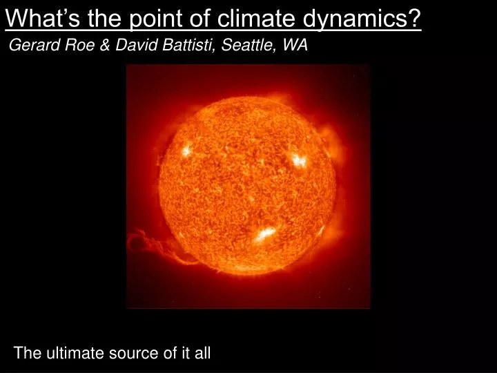
What’s the point of climate dynamics? Gerard Roe & David Battisti, Seattle, WA The ultimate source of it all

Its quite big… (NASA, TRACE)

80 S 60 S 40 S 20 S 0 20 N 40 N 60 N 80 N and shiny… Firstly, the fix on the annual mean, and look at the radiation budget Incoming solar flux (daily average top of atmosphere) W m-2  Percent reflected (top of atmosphere albedo) % ~30% latitude [Peixoto and Oort, 1992]

80 S 60 S 40 S 20 S 0 20 N 40 N 60 N 80 N Annual mean radiation budget Amount solar absorbed Q0(1-a): Amount of longwave emitted to space, F: W m-2  conv. conv. The difference: divergence [n.b. diff. tops out at 100 W m-2 high latitudes; more typically ~30-50Wm-2 latitude • surplus of energy in low latitudes, deficit in high latitudes. • this radiation imbalance drive climate dynamics. [Peixoto and Oort, 1992]

Seasonal cycle: Daily mean insolation at top of atmosphere • peaks at poles in • summer solstice. • is zero at poles at • winter solstice. • - global average • ~ 342 Wm-2 latitude month Hartmann, 1994

80 S 60 S 40 S 20 S 0 20 N 40 N 60 N 80 N Northern summer radiation budget (Jun. Jul. Aug.) Amount solar absorbed Q0(1-a): Amount of longwave emitted to space, F: W m-2  The difference: latitude [n.b. on seasonal time scales also have to worry about storage] [Peixoto and Oort, 1992]

Northern winter radiation budget (Dec. Jan. Feb.) 80 S 60 S 40 S 20 S 0 20 N 40 N 60 N 80 N Amount solar absorbed Q0(1-a): Amount of longwave emitted to space, F: W m-2  The difference: latitude [Peixoto and Oort, 1992]

Back to annual mean picture dynamical heat flux • except at high latitudes, convergence/divergence small (~20%), • compared to radiation terms • - “Climate is 80% radiation and 20% dynamics” - worth seeing how far radiation picture of climate can get you. Hartmann, 1994

Three lectures: outline Try to build up a default picture of our understanding of climate dynamics, to put climate records, and climate challenges in context. This lecture, think about radiation balance at a point (i.e., climate without dynamics). Can get demonstrate some very basic properties of climate: - climate sensitivity - climate feedbacks - timescale of climate variability These are fundamental to climate, dynamic systems in general, and hold in much more complicated (and realistic systems). “95% of climate can be explained by these processes” (Axel Timmermann) Secondly, an area in which there is huge amounts of confusion…

U.S. National Research Council report, 2003 Defines climate feedbacks incorrectly!

Three lectures: outline 2nd lecture (David) What is our basic, default understanding of role of dynamics for a) climatology? b) seasonality? c) variability? - Paleoclimate motivation: “Past is prologue” - Dynamics perspective: “The present is precedent” - Perhaps the best starting point for how things might have worked in the past is how things work today?

Three lectures: outline 3rd lecture (joint and everyone) Where is this default picture of climate dynamics challenged? • When particular climate proxy records are considered: • is it likely the proxy record can be explained using this default • picture? • Or, • does the proxy record compel us to change (i.e., advance) • our understanding Candidate examples (us, plus)

1. Climate at a point: the simplest model Let: Q0 = incident radn, a = albedo S = absorbed solar radiation and [T in oC] F = outgoing infra-red radiation: [n.b. if T F] Obtain climate from energy balance: Solve for T: Typical values: Q0=340 Wm-2, a=0.3, A=200 Wm-2, B=2 Wm-2oC-1 T = 19oC (c.f. 15oC not too shabby)

1. Climate at a point: the response to a radiative forcing, DN Question: How does the climate change? Define climate sensitivity,l, to create an objective measure of the system response to forcing: [l is change in T per unit change in N] Old climate: New climate: [this is a difference eqn for adjustment of F,S to radn forcing] Take difference:

1. Climate at a point: the response to a radiative forcing, DN Perturbation balance: Taylor series in temperature to 1st order: And so, climate sensitivity is: For our world, , so [()0 denotes reference climate model. ] Typical numbers: B=2 W m-2 oC-1  l0=0.5 oC/Wm-2 (2 x CO2  4 Wm-2 at tropopause  DT = l0DN = 2oC)

2. Climate at a point: what if there is a feedback? input output System (e.g., climate!) e.g., microphone  amplifier speaker Question: what is a feedback? Answer: an interaction where the input to a system is a partial function of the output from the system. (= hearing loss) [n.b. a feedback is only meaningfully defined in terms of a reference system without that feedback (hence the switch)]

2. Climate at a point: what if there is a feedback? Propose albedo feedback: e.g., T  i.e., let a be a function of T: Input, S, now a fn of output, T  is a feedback Revisit radn balance eqn now with extra term: Rarrange for DT: Gives new climate sensitivity:

3. Climate at a point: some terminology Defining a system Gain, G, provides an objective measure of the climate response to feedbacks Defn of Gain: In our world: [i.e. a 1% change in  per 1oC change in T] Example: suppose  = 0.3 x (1-0.01T) For our typical numbers gives G  2. Allowing an albedo feedback has doubles the sensitivity of our climate to a change in forcing!

3. Climate at a point: some terminology G 1 1 Define a feedback factor So, in our world, albedo feedback factor is [n.b. G2f0.5] [n.b. It can be shown from above that the feedback factor is equal to the fraction of the output which is fed back into the input (hence the name)]. Some possibilities -  f < 0  G < 1  response damped. 0 < f < 1  G > 1  response amplified. f > 1  G undefined  planet explodes/melts. f [n.b. the maths has gone weird b/c we assumed a new equilibrium existed with the change in forcing, which is not true in a catastrophic runaway +ve feedback (AND you have forgotten some physics)].

4. Climate at a point: what if there is more than one feedback? Suppose longwave radiation is also affected by water vapor, q, and cloud fraction, fc: That is F = F(T,q,fc) - What is the total response of the system to combined feedbacks? Previous radn balance eqn: Now, we have partial derivatives to deal with: Rearranging… Hence [n.b. The crux is that the partial derivatives appear in the denominator]

4. Climate at a point: what if there is more than one feedback? For general variables, xi: Or, can write where [n.b. fi is a function of l0, and hence depends on the reference climate state] Crucial point #1 Individual feedback factors combine linearly for total response,whereas individual gains definitelydo not combine linearly!

4. Climate at a point: what if there is more than one feedback? • Example 1 • suppose water vapor enhances response by 50%  G=1.5, f=1/3 • suppose alb. fdbck. enhances response by 100%  G=2.0, f=1/2 Linear combination of G would be 1 + 0.5 + 1.0 = 2.5 Actual = 6.0 [i.e., more than double, because feedbacks reenforce] Example 2: -two cases where the two gains would cancel: Case A: G1=1.2, G2=0.8 Case B: G1=1.8, G2=0.2 f1=1/6, f2 = -1/4 f1=4/9, f2=-4 GT=12/13  0.92 GT=9/41  0.22 Case B much more strongly damped than case A:

5. Climate at a point: time dependence Allow for storage of heat: (& warming/cooling) C = heat capacity (or thermal intertia) = mean temp. Linearize: = pert. temp. So eqn becomes But from before So get simple form:

5. Climate at a point: time dependence Let T ' = T0 at t = 0 Governing eqn has solution where • is the response timescale of the system to a perturbation i.e., the characteristic timescale of climate variability. or, equivalently  is ‘memory’ of the system - the duration over which it retains information about previous states.

5. Climate at a point: time dependence More on characteristic timescale: Crucial point #2 Four fundamental properties of the climate system - the characteristic timescale of climate variability, the thermal inertia of the system, the climate sensitivity, and climate feedbacks - are all intrinsically and tightly linked to each other [c.f. ei = -1]. Crucial point #3 It is a very strong expectation that this relationship applies to most aspects of the climate system - (fundamental to all dynamic systems).

6. Climate at a point: the effect of random noise Can always expect random noise in the climate system: What is the effect of this noise on the behavior of the system? For time dep. eqn with random noise, dN’: rearranging Random forcing drives T' away from eqm. restoring ‘force’ - a relaxation back to equilibrium (T'=0)

6. Climate at a point: the effect of random noise Discretize eqn into time steps, t: Equation becomes where t is white noise current state random noise memory of last state - How does the system’s response to noise vary as a function of the memory,  = (l,C, fi)?

6. Climate at a point: the effect of random noise t = 5 yrs t = 1 yr t = 25 yrs Time (yrs) The effect of varying t on the response of T’ to forcing by noise. note multi-decadal excursions here note century-scale excursions here The greater the memory, the longer the timescale of the variability

6. Climate at a point: the effect of random noise Climate is defined the statistics of weather. (i.e. the mean and standard deviation of atmospheric variables) Therefore a constant climate has a constant standard deviation (i.e., even in a constant climate there is variability) Crucial point #4: In paleoclimate, if the proxy variable (i.e., glacier, lake, tree, elephant, etc.) has long memory, say, t ~ 25 yrs, that proxy will have long timescale (i.e., centennial) variability even in a constant climate.

7. Climate at a point: power spectrum of response to noise amplitude time log(power) log(period=1/frequency) Quick intro to power spectra: they are an alternative way of describing a time series Time series Power spectrum Gives power (energy) at each sine wave frequency that makes up the time series (analogous to spectrum of light)

7. Climate at a point: power spectrum of response to noise t =1 yr log(power) t =5 yrs t =25 yrs log(period=1/frequency) Power spectra of response to noise as a function of t As  there is more damping at high frequencies • The long t is, the ‘redder’ the power spectrum, • i.e., the greater the relative amount of long period variability.

7. Climate at a point: power spectrum of response to noise t =1 yr log(power) t =5 yrs t =25 yrs log(period=1/frequency) Eqn for this power spectra t • Can show 50% of power • in the spectrum occurs at • periods which are greater • than2 x . t t Crucial point #5 Long period variability is driven by short timescale physics.

7. Climate at a point: power spectrum of response to noise Why the factor of 2? i) Hand-wavy analogy with pendulum: Physical timescale Oscillation period ii) Real reason: Real time-behavior ~ Projected onto sines and cosines ~

8. Example: the Pacific Decadal Oscillation Dominant pattern of sea surface temperatures in North Pacific

8. Example: the Pacific Decadal Oscillation Power spectrum of PDO index Lots of variability at multi-decadal time scale But…. Best fit is a red noise process with a  of 1.20.3 years i.e., indistinguishable from an annual timescale.

8. Example: the Pacific Decadal Oscillation PDO index Random noise & 1.2yr memory Random noise & 1.2yr memory [n.b. note the apparent long timescale variability even with short memory]

Summary: • get definitions of feedbacks right! • , l, C,and fi are all inextricably intertwined. • robust property of natural, nonlinear dynamical systems. • if a climate proxy has memory, expect long timescale variations • even if climate is not changing. • changes the question from what was the climate change • to was there a climate change? • Long period variability is driven by short timescale physics, • default expectation is that multi-decadal variability comes from • sub-decadal physics!

Small print: In general, feedback strengths and sensitivity are functions of the mean state: For a black-body [Stefan-Boltzmann law] We linearized into A+BT: Our basic climate sensitivity: l0=1/B, is a sensitive function of T. Feedback analyses are completely linear, can be trouble when strongly nonlinear behavior is being studied. Feedback analyses rely on defining an appropriate reference state, against which to test models/observations. You have to be careful that the same reference state is being use when comparing feedbacks.

What’s the point of climate dynamics?