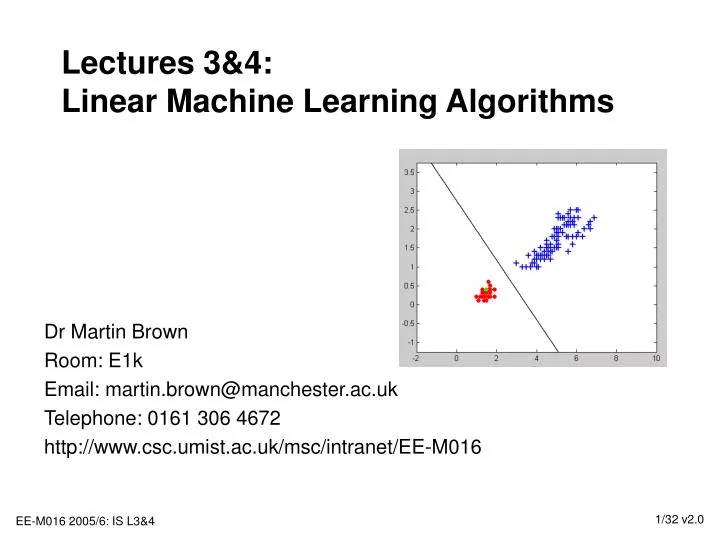
Lectures 3&4: Linear Machine Learning Algorithms

Lectures 3&4:Linear Machine Learning Algorithms Dr Martin Brown Room: E1k Email: martin.brown@manchester.ac.uk Telephone: 0161 306 4672 http://www.csc.umist.ac.uk/msc/intranet/EE-M016

Lectures 3&4: Outline • Linear classification using the Perceptron • Classification problem • Linear classifier and decision boundary • Perceptron learning rule • Proof of convergence • Recursive linear regression using LMS • Modelling and recursive parameter estimation • Linear models and quadratic performance function • LMS and NLMS learning rules • Proof of convergence

Lectures 3&4: Learning Objectives • Understand what classification and regression machine learning techniques are and their differences • Describe how linear models can be used for both classification and regression problems • Prove convergence of the learning algorithms for linear relationships, subject to restrictive conditions • Understand the restrictions of these basic proofs • Develop basic framework that will be expanded on in subsequent lectures

Lecture 3&4: Resources • Classification/Perceptron • An introduction to Support Vector Machines and other kernel-based learning methods, N Cristianini, J Shawe-Taylor, CUP, 2000 • Regression/LMS • Adaptive Signal Processing, Widrow & Stearns, Prentice Hall, 1985 • Many other sources are available (on-line).

What is Classification? • Classification is also known as (statistical) pattern recognition • The aim is to build a machine/algorithm that can assign appropriate qualitative labels to new, previously unseen quantitative data using a priori knowledge and/or information contained in a training set. The patterns to be classified are usually groups of measurements/observations, that are believed to be informative for the classification task. • Example: Face recognition Training data: D = {X,y} Prior knowledge Design/ learn Classifier m(q,x) ^ Predict ^ Predicted class label: y New pattern: x

Classification Training Data • To supply training data for a classifier, examples must be collected that contain both positive (examples of the class) and negative (examples of other classes) instances. These are qualitative target class values and are stored as +1 and -1, for the positive and negative instances respectively. Generated by expert or by observation. • The quantitative input features should be informative • The training set should contain enough examples to be able to build statistically significant decisions How to encode qualitative target and input features?

Bayes Class Priors • Classification is all about decision making using the concept of “minimum risk” • Imagine that the training data contains 100 examples, 70 of them are class 1 (c1), 30 are class 2 (c2) • If I have to decide which class an unknown example belongs to, which decision is optimal? • Errors if decision is class 1: p(c1) = • Errors if decision is class 2: p(c2) = • Minimum risk decision is: • p(c1) & p(c2) are known as the Bayes priors, they represent the baseline performance for any classifier. They are derived from the training data as simple percentages

Structure of a Linear Classifier • Given a set of quantitative features x, a linear classifier has the form: • The sgn() function is used to produce the qualitative class label (+/-1) • The class/decision boundary is determined when: • This is an (n-1)D hyperplane in feature space. • In 2-dimensional feature space: • How does the sign and magnitude of q affect the decision boundary? x2 + + + + + + + + x1

Simple Example: Fisher’s Iris Data • Famous example of building classifiers for a problem with 3 types of Iris flowers and 4 measurements about the flower: • Sepal length and width • Petal length and width • 150 examples were collected, 50 from each class • Build 3 separate classifiers, one for recognizing examples of each class • Data is shown, plotted against last two features, as well as two linear classifiers for the Setosa and Virginica classes Calculate q in lab 3&4 …

Perceptron Linear Classifier • The Perceptron linear classifier was devised by Rosenblatt in 1956 • It comprises a linear classifier (as just discussed) and a simple parameter update rule of the form: • Cyclically present each training pattern {xk, yk} to the linear classifier • When an error (misclassification) is made, update the parameters: • where h>0 is the learning rate. • The bias term can be included as q0 with an extra feature x0 = 1: • Continue until there are no prediction errors • Perceptron convergence theorem If the data set is linearly separable, the perceptron learning algorithm will converge to an optimal separator in a finite time

^ xTq Instantaneous Parameter Update • What does this look like? • The parameters are updated to make them more like the incorrect feature vector. • After updating: • Updated parameters are closer • to correct decision x2, q2 ^ Error-driven update: ^ x1, q1 ^ y, y 1 0 -1

Perceptron Convergence Proof Preamble … • Basic aim is to minimise the number of mis-classifications: • This is generally an NP-complete problem • We’ve assumed that there is an optimal solution with 0 errors • This is similar to Least Squares recursive estimation: • Performance = Si(yi-yi)2 = 4*numberOfErrors • Except that the sgn() makes it a non-quadratic optimization problem • Updating only when there are errors is the same as: • with or without errors • Sometimes drawn as a network: ^ “error driven” parameter estimation Repeatedly cycle through data set D, drawing out each sample {xk, yk} ^ yk xk - + yk

Convergence Analysis of the Perceptron (i) • If a linearly separable data set D is repeatedly presented to a Perceptron, then the learning procedure is guaranteed to converge (no errors) in a finite time • If the data set is linearly separable, there exists optimal parameters q such that for all i = 1, …, l • Note that are also optimal parameter vectors • Consider the positive quantity g defined by, such that ||q|| = 1: • This is a concept known as the “classification margin” • Assume also that the feature vectors are bounded by:

Convergence Analysis of the Perceptron (ii) • To show convergence, we need to establish that at the kth iteration, when an error has occurred: • Using the update formula: q2 ^ qk ^ qk+1 q q1 To finish proof, select

Convergence Analysis of the Perceptron (iii) • To show this terminates in a finite number of iterations, simply note that: • is independent of the current training sample, so the parameter error must decrease by at least this amount at each update iteration. As the initial error is finite, q0 = 0, say, there must exist a finite number of steps before the parameter error is reduced to zero. • Note also that a is proportional to the size of the feature vector (R2) and inversely proportional to the size of the margin (g). Both of these will influence the number of update iterations when the Perceptron is learning ^

Example of Perceptron (i) • Consider modelling the logical AND data using a Perceptron Is the data linearly separable? ^ ^ ^ k=0, q = [0.01, 0.1, 0.006] k=5, q = [-0.98, 1.11, 1.01] k=18, q = [-2.98, 2.11, 1.01] x2 x2 x2 x1 x1 x1

^ q1,k ^ ^ qi,k q2,k ^ bias q0,k k: data presentation index Example: Parameter Trajectory (ii) Lab exercise: Calculate by hand the first 4 iterations of the learning scheme

Classification Margin • In this proof, we assumed that there exists a single, optimal parameter vector. • In practice, when the data is linearly separable, there are an infinite number – simply requiring correct classification results in an ill-posed posed problem • The classification margin can be defined as the minimum distance of the decision boundary to a point in that class • Used in deriving Support Vector Machines x2 x1 x2 1 0 -1 x1

Classification Summary • Classification is the task of assigning an object, described by a feature vector, to one of a set of mutually exclusive groups • A linear classifier has a linear decision boundary • The perceptron training algorithm is guaranteed to converge in a finite time when the data set is linearly separable • The final boundary is determined by the initial values and the order of presentation of the data

Definition of Regression • Regression is a (statistical) methodology that utilizes the relation between two or more quantitative variables so that one variable can be predicted from the other, or others. • Examples: • Sales of a product can be predicted by using the relationship between sales volume and amount of advertising • The performance of an employee can be predicted by using the relationship between performance and aptitude tests • The size of a child’s vocabulary can be predicted by using the relationship between the vocabulary size, the child’s age and the parents’ educational input.

rmse = s Regression Problem Visualisation • Data generated by • Estimate model parameters • Predict a real value (fit a curve to the data) • Predictive performance • average error + + + + + ^ ^ + y, y y + + + + + + + + + + + + + + + + + x

y, y + + + m(y|x) = 12 s(e) = 1.5 12 + + + + + x Probabilistic Prediction Output • An output of 12 with rmse/standard deviation = 1.5: Within a small region close to the query point, the average target value was 12 and the standard deviation within that region was 1.5 (variance = 2.25) m(y|x) = 12 ^ 2s(e) = 3 95% of the data lies in the range m+/-2s = [12 +/-2*1.5] = [9,15]

Given a set of features x, a linear predictor has the form: The output is a real-valued, quantitative variable The bias term can be included as an extra feature x0 = 1. This renames the bias parameter as q0. Most linear control system models do not explicitly include a bias term, why is this? Similar to the Toluca example in week 1. ^ y, y x Structure of a Linear Regression Model

Least Mean Squares Learning • Least Mean Squares (LMS) proposed by Widrow 1962 • This is a (non-optimal) sequential parameter estimation procedure for a linear model: • NB, compared to classification, both yk and yk are quantitative variables, so the error/noise signal (yk-yk) is generally non-zero. Similar to the Perceptron, but no threshold on xTq. h is again the positive learning rate. • Widely used in filtering/signal processing and adaptive control applications • “Cheap” version of sequential/recursive parameter estimation • The normalised version (NLMS) was developed by Kaczmarz in 1937 ^ ^ ^

Proof of LMS Convergence (i) • If a noise-free data set containing a linear relationship x->y is repeatedly presented to a linear model, then the LMS algorithm is guaranteed to update the parameters so that they converge to their optimal values, assuming the learning rate is sufficiently small. • Note: • Assume there is no measurement noise in the target data • Assume the data is generated from a linear relationship • Parameter estimation will take an infinite time to converge to the optimal values • Rate of convergence and stability depend on the learning rate

q2 ^ qk ^ qk+1 q q1 Proof of Convergence (ii) • To show convergence, we need to establish that at the kth iteration, when an error has occurred: • Using the update formula: when

Example: LMS Learning • Consider the “target” linear model y = 1 - 2*x, where the inputs are drawn from a normal distribution with zero mean, unit variance • Data set consisted of 25 data points, and involved 10 cycles through the data set • h=0.1 k=100 y, y k=5 ^ k=0 x ^ q0 ^ ^ q q1 ^ q1 ^ q0 k

Stability and NLMS • To normalise the LMS algorithm and remove the dependency of h on the input vector size, consider: • This learning algorithm is stable for 0<h< 2 (exercise). • When h=1, the NLMS algorithm has the property that the error, on that datum, after adaptation is zero, ie: • Exercise: prove this. • Is this desirable when the target contains (measurement) noise?

Regression Summary • Regression is a (statistical) technique for predicting real-valued outputs, given a quantitative feature vector • Typically, it is assumed that the dependent, target variable is corrupted by Gaussian noise, and this is unpredictable. • The aim is then to fit the underlying linear/non-linear signal. • The LMS algorithm is a simple, cheap gradient descent technique for updating the linear parameter estimates • The parameters will converge to their correct values when the target does not contain any noise, otherwise they will oscillate in a zone around the optimum. • Stability of the algorithm depends on the learning rate

Lecture 3&4: Summary • This lecture has looked at basic (linear) classification and regression techniques • Investigated basic linear model structure • Proposed simple, “on-line” learning rules • Proved convergence for simple environments • Discussed the practicality of the machine learning algorithms • While these algorithms are rarely used in this form, their structure has strongly influenced the development of more advanced techniques • Support vector machines • Multi-layer perceptrons • which will be studied in the coming weeks

Laboratory 3&4: Perceptron/LMS • Download the irisClassifier.m & iris.mat Matlab files that contain a simple GUI for displaying the Iris data and entering decision boundaries • Enter parameters that create suitable decision boundaries for both the Setosa and Virginica classes • Which of the three classes are linearly separable? • Make sure you can translate between the classifiers’ parameters, q, and the gradient/intercept coordinate systems. Also ensure that the output is +1 (rather than -1) in the appropriate region • Download the irisPerceptron.m and perceptron.m Matlab files that contain the Perceptron algorithm for the Iris data • Run the algorithm and note how the decision boundary changes when a point is correctly/incorrectly classified • Modify the learning rate and note the effect it has on the convergence rate and final values

Laboratory 3&4: Perceptron/LMS (ii) • Copy and modify the irisPerceptron.m Matlab file so that it runs on the logical AND and OR classification functions (see slides 16 & 17). Each should contain 2 features and four training patterns. Make sure you can calculate the updates by hand, as required on Slide 17. • Create a Matlab implementation of example given in Slide 27 for the LMS algorithm with a simple, single input linear model • What values of h causes the LMS algorithm to become unstable? • Can this ever happen with the Perceptron algorithm? • Modify this implementation to use the NLMS training rule • Verify that learning is always stable for 0 < h < 2. • Complete the two (pen and paper) exercises on Slide 28. • How might this insight be used with the Perceptron algorithm to implement a dynamic learning rate?

Lectures 3&4: Linear Machine Learning Algorithms