Download
1 / 34
340 likes | 470 Views
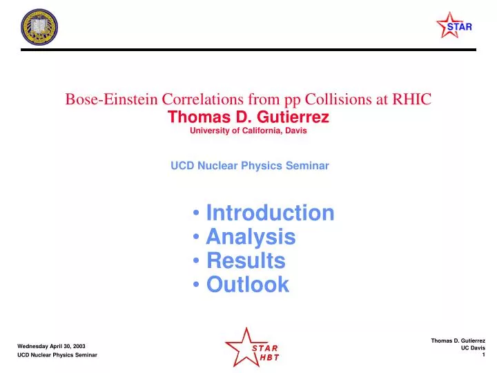
Bose-Einstein Correlations from pp Collisions at RHIC Thomas D. Gutierrez University of California, Davis. UCD Nuclear Physics Seminar. Introduction Analysis Results Outlook. P1. r A1. r B1. R. r A2. d. P2. r B2. L >> (d & R). What are Bose-Einstein Correlations?.

E N D
Bose-Einstein Correlations from pp Collisions at RHIC Thomas D. Gutierrez University of California, Davis UCD Nuclear Physics Seminar • Introduction • Analysis • Results • Outlook
P1 rA1 rB1 R rA2 d P2 rB2 L >> (d & R) What are Bose-Einstein Correlations? Bose-Einstein correlations (BEC) are a joint measurement of more than one boson in some variable of interest. For example, if the variable of interest is momentum then information about the geometry of boson emission source can be obtained (more on this later) In its simplest form, BEC often predicts an enhancement of boson coincident counts (relative to the experiment performed with non-bosons). This is usually associated with Bose-Einstein statistics. But things are rarely this simple. BEC often goes under the name HBT or GGLP. I’ll use HBT.
What is HBT? The technique was originally developed by two English astronomers Robert Hanbury-Brown and Richard Twiss (circa 1952) It’s a form of “Intensity Interferometry” -- as opposed to “regular” amplitude-level (Young or Michelson) interferometry -- and was used to measure the angular sizes of stars The method had far reaching consequences! A quantum treatment of HBT generated much controversy and led to a revolution in quantum optics Later it was used by high energy physicists to measure source sizes of elementary particle or heavy ion collisions (the GGLP effect) But how does HBT work? And why use it instead of “regular” interferometry?
rA1 P1 A Plane wave rB1 d Monochromatic Source B L >> d (brackets indicate time average -- which is what is usually measured) Two slit interference (between coherent sources at A and B) “source geometry”(d) is related to interference pattern
A d B L >> d (brackets again indicate time average) “Two slit interference” (between incoherent sources at A and B) P1 rA1 Two monochromatic but incoherent sources (i.e.with random, time dependent phase) produce no interference pattern at the screen -- assuming we time-average our measurement over many fluctuations rB1
P1 rA1 rB1 R rA2 d P2 rB2 L >> (d & R) HBT Example (incoherent sources) As before... A But if we take the product before time averaging... B where Important: The random phase terms completely dropped out. We can extract information about the source geometry!
Increasing angular size Increasing source size d Notice that the “widths” of these correlation functions are inversely related to the source geometry source Width w A source can also be a continuous distribution rather than just points The width of the correlation function will have a similar inverse relation to the source size Width ~1/w Correlation function Astronomy For fixed k Particle physics I’ll drop
More About HBT Than is probably healthy As we’ve seen, when treated with classical waves, HBT is basically just a kind of beat phenomenon When treated quantum mechanically (i.e. actually counting particles) the situation is more complex Lets define the two particle correlation function as: The density matrix in the second expression tells us two very important things: C2 is sensitive not only to the quantum statistics (determined by the commutation relations of the a and a’) but also the quantum field configuration; C2 is sensitive to the source distribution, the dynamics of the problem, as well as any space-momentum correlations
Joint probability of measuring a particle at both detectors 1 and 2 Measuring the correlation function is really just a counting game Probability of measurement at 1 times probability of a measurement at 2 Note: if the two measurements are statistically independent then C2=1 C2 Thermal Bosons 2 Two quantum field configurations of interest: coherent state (like a “laser”) and thermal state (following a Bose-Einstein distribution) Partly coherent bosons+thermal+contamination Chaoticity parameter C2 is often measured as a function of the momentum difference and can often be parameterized like a Gaussian: ~ 1/R 1 Totally coherent Q=|p1-p2| Momentum difference Non-interacting fermions 0 Sill more about HBT Than is probably healthy
Practicalities of HBT Interferomertry using particles in HEP • Compare relative 4-momenta (Qinv) of identical particles (e.g. pions) to determine information about space-time geometry of source. • Experimentally, 1D C2 correlation functions are created by comparing relative 4-momenta of pairs from a “real” event signal to pairs from “mixed” events. • The mixed background presumably has no HBT signal! STAR Preliminary STAR Preliminary
=0.397 +/- 0.013; Rg=1.16 fm +/- 0.032; =0.749 +/- 0.030; Re=1.94 fm +/- 0.071 More HBT practicalities in HEP • The correlation function, C2, is created by dividing the “real” pairs by “mixed” pairs. The histogram is then normalized to the baseline. • The data are fit to a Gaussian or an exponential to extract fit parameters Rinv and λ. C2g = 1 + λexp(-Qinv2Rinv2) C2e = 1 + λexp(-QinvRinv) STAR Preliminary ~λe ~1/R Both fits are to the Coulomb corrected data (dark blue) The Coulomb repulsion experienced by identical charged pairs tends to deplete the correlation function at low Q -- this can be corrected
π+/p NA22 e+/e- AMY E735 UA1 OPAL Why study HBT in pp Collisions? • There is a long history of doing Bose-Einstein pion correlations in elementary particle collisions • In the context of RHIC, it provides a baseline for the heavy ion results Just a sampling • Dowell., Proc. Of the VII Topical Workshop on Proton-AntiProton Collider Physics, p115, Word Scientific 1989. • Lindsey. “Results from E735 at the Tevetron Proton-AntiProton Collider with root s= 1.8TeV”, Presented at the Quarkmatter 1991, Gatlinberg, Tennessee, Nov 11-15, 1991. • OPAL Collaboration. Physics Letters B. Vol 267 #1, 5 September, 1991. • NA22 Collaboration “Estimation of Hydrodynamical model parameters from the invariant spectrum and the Bose-Einstein Corrilations…”, Nijmegen preprint, HEN-405, Dec. 97. fm p/pbar
In this 1D inside-out fragmentation picture, rapidity and z are correlated. Particles near each other in rapidity, will also be near each other in space. Particles close in space and momentum contribute most strongly to the HBT signal For non-static sources, HBT becomes sensitive to regions of homogeneity; this gives rise to a phase space dependence of the radii N K HBT radii will often be much smaller than actual hadronization surface What is HBT Actually Measuring? t y2 y1 Hadronization “freeze out” surface (mean) Quark scattering and creation z Regions of Homogeneity P T
HBT Study of the pp System • HBT studies in pp interactions provide a peek into the fascinating soft-physics regime of hadronic collisions • Some HBT-related questions: • What do the regions of homogeneity look like? • What is the pair source distribution function? • How do the HBT parameters depend on event multiplicity? • Do the HBT parameters depend on the polarization of the initial state (a fun idea but won’t have time to talk about it today)? This analysis is a first step in answering some of these questions
The STAR Experiment STAR main detector: Time Projection Chamber (a large-acceptance cylindrical detector) E field and B field along the beam direction. 12 million reversed full field and full field, minimum bias pp events at 200GeV from RHIC using the STAR detector; some data presented include only the 7 million RFF Particle identification done by measureing dE/dx (specific energy loss)
Track and Event Selection (I) • For negative and positive pions at two mid-rapidity ranges (-0.5<y<0.5; -1<y<1), four kt ranges were analyzed (0.15<kt<0.25, 0.25<kt<0.35, 0.35<kt<0.45, 0.45<kt<0.65 GeV/c) • Particle identification was done by taking a one sigma cut around the pion bethe-bloch curve while excluding other particles at the two sigma level. dEdx vs. P (GeV/c) STAR Preliminary Kt is the average PAIR transverse moment similar Y is the TRACK rapidity
Track and Event Selection (II) • Some additional cuts used for this analysis • Verices accepted 3m across the STAR TPC • Analysis done separately for 20cm wide regions (results then added) • For the non-multiplicity dependent analyses: event Multiplicity < 30 • Analysis performed separately for like-multiplicity events (results then added) • Only accept events with at least 2 tracks • Track level • -0.5 < y < 0.5 and -1<y<1 • PID cuts as discussed • Primary tracks only • Pair level • Four kt bins between: 0.15 < kt <0.65 GeV/c • anti-merging and anti-splitting cuts applied STAR Preliminary pass fail zvertex The effects of pileup in pp have not yet been studied in the context of HBT The first order effect would be to reduce the lambda factor (a pileup would act like a mixed event thus “watering down” the signal)
Pair Cuts (I): Track Merging -0.5<y<0.5 -1<y<1 STAR Preliminary STAR Preliminary Accept >9cm Accept > 9cm 0.15 < kt <0.65 GeV/c for Qinv<0.2 GeV/c The above correlation functions are a measure of track merging (2 tracks mistaken as one) relative to a mixed background which presumably has no track merging looks similar
Pair Cuts (II): Track Splitting -0.5<y<0.5 Splitting is when one track is mistaken as 2 STAR Preliminary Pads with two hits are circled Accept -0.5<Quality<0.6 Qual~0 no splitting (really DO have 2 tracks) Qual=1 totally split (one track mistaken as 2) 0.15 < kt <0.65 GeV/c The above correlation function is a measure of the quality relative to a mixed background. The mixed background presumably has no splitting (high quality means more splitting) and +/- 1 y looks similar
1D Qinv Correlation Functions (I) All fits are to the Coulomb corrected data: The pi+ pi- combined over -1<y<1 will serve as the standard All plots here 0.15<kt<0.25 GeV All STAR Preliminary
1d Qinv Correlation Functions (II) The strength of this high Qinv tail depends on the kinematic cuts; The effect is currently under study The traditional Gaussian fit (black) isn’t very good; The exponential fits do much better; various parameterizations are under study All plots here 0.15<kt<0.25 GeV; -1<y<1; pi+ and pi- All STAR Preliminary
Pythia pi- (no afterburner); 0.15<pt<1.1; -0.5<y<0.5; 1M events; ignore normalization; evidence of some sloping; will perform a more systematic study C2 Baseline curvature depends only very weakly on particle species and zvertex choices; depends more strongly on rapidity and kt cuts; Still a rather small effect overall The current hypothesis is that the effect is due to energy-momentum conservation Qinv 1D Qinv Correlation Functions (III) All STAR Preliminary All plots here 0.15<kt<0.25 GeV;
R (fm) 1D Qinv HBT Parameters All are from 0.15<kt<0.25 GeV; -1<y<1; pi+ and pi- Highly parameterization dependent values = bad
is the pair wavefunction and includes all the appropriate quantum statistics and relevant interactions between the pair Source Image Another interesting way to approach HBT is one can transform the correlation function to obtain the actual source numerically Thermal limit: Koonin-Pratt equation S is the source distribution and represents the probability of emitting a pair of particles with relative 4-momentum=Qinv separated by a distance r; S is the quantity we want to extract K0 is the angle averaged integration kernel and is given by
Source Image C2 log(S) STAR Preliminary 0.15<kt<0.25; -0.5<y<0.5; pi- Qinv Reconstructed correlation function; red is the non- Coulomb corrected input Qinv Correlation function Pair source emission function S(r); log scale Qinv r (fm) Generated using Brown and Danielewicz's HBTprogs v.1.0 ` The different colors represent different parameters in the HBTprogs program Is there a double Gaussian structure in the source function? More work needs to be done to really determine this. A promising method: still a work in progress
y x y x 3D Correlation Functions By looking at a 3D correlation function we can extract a more complete picture of the source.
3D Correlation Functions kt cut with ~0.15 GeV/c pid pt cut causes Qout “hole” y cuts cause Qlong “cutoff” C2 All plots here 0.15<kt<0.25 GeV; -1<y<1; pi+ and pi- side out long C2 = N[1 + λexp(-qout2Rout2 -qside2Rside2 -qlong2Rlong2)] Fits and correlations projected 80MeV in the “other” directions All STAR Preliminary
Rout Rside Rlong 3D Correlation Parameters C2 = N[1 + λexp(-qout2Rout2 -qside2Rside2 -qlong2Rlong2)] 0.15<kt<0.25 GeV; -1<y<1; pi+ and pi-
AuAu 200GeV Central Midcentral Peripheral M. Lopez-Noriega QM2002 3D Correlation Functions: kt dependence STAR Preliminary Rlong Rside Rout R(fm) kt kt What causes kt dependence?
Kt = pair Pt Not all of these will give the same kt dependence. The trick is in distinguishing between them. This is currently under study Rside Rout What Causes Kt Dependence? Space momentum correlations Space momentum correlations Space momentum correlations We are looking at a region of homogeneity caused by: If the source is not static or collective effects are present then space-momentum correlations can develop and cause the radii to change as you look in different locations in phase space. Some examples Inside-out fragmentation/ hadronization jets (the ultimate space-momentum correlation) fireball-like expansion collective flow
Multiplicity Dependence of HBT parameters It has been reported by some experiments (e.g. UA1 ppbar at 630 GeV) that lambda tends to drop with event multiplicity while the radius increases slowly Other experiments (e.g. NA27 pp at 27 GeV) report that lambda is flat as a function of event multiplicity This puzzle has numerous explanations from the mundane to the exotic. Some current speculations: Pion emission becomes more coherent in high multiplicity events involving particle-antiparticle collisions but not particle-particle High multiplicity events from ppbar may involve multistring fragmentation -- pions from different strings will not correlate strongly Resonance contributions and other contaminates may contribute to different degrees at different multiplicities at different experiments All of the above would have the tendency to reduce lambda
Multiplicity dependence of 1D HBT Using full RFF+FF This preliminary STAR pp result indicates lambda is flat as a function of event multiplicity STAR Preliminary STAR Exponential NA27, NA23, and NA22 all reported similar results NA27 pp 27 GeV (Gaussian) STAR Gaussian This is clearly not the case at UA1 UA1 ppbar 630 GeV (Gaussian) • NA27 ZPC 54,21 1992 • UA1 PLB 226, 410, 1989 charged Very Important: Not corrected for resonances or efficiency Low multiplicity bins (<4) have large systematic error bars -- still being studied
Multiplicity Dependence of 1D Radius STAR Preliminary • NA27 ZPC 54,21 1992 • UA1 PLB 226, 410, 1989 This preliminary STAR pp result indicates rinv is flat as a function of event multiplicity STAR Exponential STAR Gaussian Very Important: Not corrected for resonances or efficiency Low multiplicity bins (<4) have large systematic error bars -- still being studied
Summary Bose-Einstein correlations provide a means of probing the space-time geometry of the pion emission source in high energy collisions; The pion emission source size is ~1 fm A kt dependence is seen in the 3D HBT parameters of pp collisions indicating a pion source with space-momentum correlations; The nature of ths source is still under study Lambda and rinv are constant as a function of event multiplicity; This is consistent with other pp experiments but differ from ppbar results; The effect is still under study