Download
1 / 19
220 likes | 611 Views
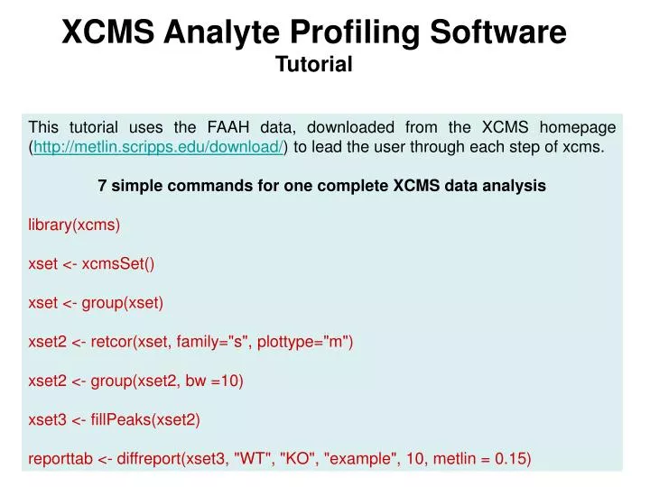
XCMS Analyte Profiling Software Tutorial. This tutorial uses the FAAH data, downloaded from the XCMS homepage ( http://metlin.scripps.edu/download/ ) to lead the user through each step of xcms. 7 simple commands for one complete XCMS data analysis library(xcms) xset <- xcmsSet()

E N D
XCMS Analyte Profiling SoftwareTutorial This tutorial uses the FAAH data, downloaded from the XCMS homepage (http://metlin.scripps.edu/download/) to lead the user through each step of xcms. 7 simple commands for one complete XCMS data analysis library(xcms) xset <- xcmsSet() xset <- group(xset) xset2 <- retcor(xset, family="s", plottype="m") xset2 <- group(xset2, bw =10) xset3 <- fillPeaks(xset2) reporttab <- diffreport(xset3, "WT", "KO", "example", 10, metlin = 0.15)
Open R, load xcms User input is shown in red
Go to File toolbar at the top of R, choose Change dir…, and select the folder containing the .cdf files
Upload data files xset is a user defined object name Upload data files completed
Check loaded data; this step is optional and does not affect data analysis.
Or add sleep = .001 to the group command for grouping peaks with visualization
Retention time correction The retcor command can either be typed out completely i.e. using family = “symmetric”, plottype = “mdevden” or simply as family = “s”, plottype = “m”. Note: the object name ‘xset2’ is used here, so that the original xset will not be overwritten.
Fill in with original data where peaks were not detected initially. Note: the object name xset3 is used here, so that xset2 and xset will not be overwritten.
Check current data status; this step is optional and does not affect data analysis.
Create report: • “WT” and “KO” denote the class names of the data sets being compared • “example” is a user defined output file name for the spreadsheet report • 10 is a user defined number of extracted ion chromatograms (EIC) that will be plotted • metlin = 0.15 specifies the m/z tolerance for potential metabolite matches from the METLIN database
Both the EICs and spreadsheet report (as a TSV file) are created in the same folder where the raw data are stored
Inside the EIC folder. EICs can also be visualized in many picture viewing programs
Type ? before the function name to retrieve documentation immediately i.e. ?retcor will bring up the retention time correction documentation page.
All the functions and classes are documented and are available from R under Help > Html help > Packages > xcms.
A detailed description of XCMS is available for download in the Documentation section