Download
1 / 21
210 likes | 480 Views
Lecture #16 EGR 261 – Signals and Systems. Read : Ch. 14, Sect. 1-5; Ch. 15, Sect. 1-2; and App. D&E in Electric Circuits, 9 th Edition by Nilsson. Bode Plots - Recall that there are 5 types of terms in H(s). The first four have already been covered. 5. Complex terms in H(s)

E N D
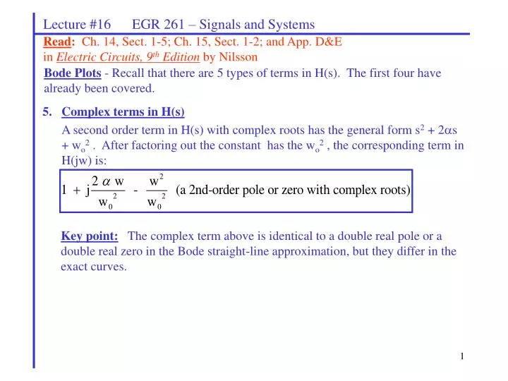
Lecture #16 EGR 261 – Signals and Systems Read: Ch. 14, Sect. 1-5; Ch. 15, Sect. 1-2; and App. D&E in Electric Circuits, 9th Edition by Nilsson Bode Plots - Recall that there are 5 types of terms in H(s). The first four have already been covered. 5.Complex terms in H(s) A second order term in H(s) with complex roots has the general form s2 + 2s + wo2 . After factoring out the constant has the wo2 , the corresponding term in H(jw) is: Key point: The complex term above is identical to a double real pole or a double real zero in the Bode straight-line approximation, but they differ in the exact curves.
Lecture #16 EGR 261 – Signals and Systems Complex peaks and damping ratio Exercise: Complete the table below showing the value of the complex peak (for a complex zero) * z = 1 is not complex. It corresponds to a double-zero.
Lecture #16 EGR 261 – Signals and Systems The following graphs from the text (Electric Circuits, 6th Edition, by Nilsson) below show the Bode straight-line approximation (Figure 14.41) and the exact curve for different values of z (Figure 14.42).
Lecture #16 EGR 261 – Signals and Systems Example: Sketch the LM responses for H1(s), which has a double zero, and H2(s), which has a complex zero. A) Find H1(jw) and sketch the LM response
Lecture #16 EGR 261 – Signals and Systems Example: Sketch the LM responses for H1(s), which has a double zero, and H2(s), which has a complex zero. B) Find H2(jw) and sketch the LM response
Lecture #16 EGR 261 – Signals and Systems Filters A filter is a circuit designed to have a particular frequency response, perhaps to alter the frequency characteristics of some signal. It is often used to filter out, or block, frequencies in certain ranges, much like a mechanical filter might be used to filter out sediment in a water line. • Basic Filter Types • Low-pass filter (LPF) - passes frequencies below some cutoff frequency, wC • High-pass filter (HPF) - passes frequencies above some cutoff frequency, wC • Band-pass filter (BPF) - passes frequencies between two cutoff frequency, wC1 and wC2 • Band-stop filter (BSF) or band-reject filter (BRF) - blocks frequencies between two cutoff frequency, wC1 and wC2
Lecture #16 EGR 261 – Signals and Systems Ideal filters An ideal filter will completely block signals with certain frequencies and pass (with no attenuation) other frequencies. (To attenuate a signal means to decrease the signal strength. Attenuation is the opposite of amplification.) LM LM Ideal LPF Ideal HPF w w wC wC LM LM Ideal BPF Ideal BSF w w wC1 wC2 wC1 wC2
Lecture #16 EGR 261 – Signals and Systems Filter order Unfortunately, we can’t build ideal filters. However, the higher the order of a filter, the more closely it will approximate an ideal filter. The order of a filter is equal to the degree of the denominator of H(s). (Of course, H(s) must also have the correct form.) LM Ideal LPF slope = 4th-order LPF slope = -80dB/dec 3rd-order LPF slope = -60dB/dec 2nd-order LPF slope = -40dB/dec 1st-order LPF slope = -20dB/dec w wC
Lecture #16 EGR 261 – Signals and Systems Low-pass filter (LPF) - Discuss the form of LM, H(jw), and H(s). High-pass filter (HPF) - Discuss the form of LM, H(jw), and H(s).
Lecture #16 EGR 261 – Signals and Systems Band-pass filter (BPF) - Discuss the form of LM, H(jw), and H(s). Band-stop filter (BSF) - Discuss the form of LM, H(jw), and H(s). Also define a “notch” filter.
Lecture #16 EGR 261 – Signals and Systems Practical Filter Examples: Discuss a stereo tuner, 5-band equalizer, FSK demodulator, 60 Hz interference block.
Lecture #16 EGR 261 – Signals and Systems Active and passive filters Passive filter - a filter constructed using passive circuit elements (R’s, L’s, and C’s) Active filter - a filter constructed using active circuit elements (primarily op amps) Analysis of active filters Active filters are fairly easy to analyze. Recall that a resistive inverting amplifier circuit has the following relationship: Replacing the resistors with impedances yields a transfer function, H(s):
Lecture #16 EGR 261 – Signals and Systems Example: Find H(s) =Vo(s)/Vin(s) for the circuit below and sketch the LM response.
Lecture #16 EGR 261 – Signals and Systems Impedance and Frequency Scaling Filter tables are commonly available that list component values for various types of filters. However, the tables could not possibly list component values for all possible cutoff frequencies. Typically, filter tables will list cutoff frequencies of perhaps 1 Hz or 1 kHz. The user can then scale the cutoff frequencies to the desired values using frequency scaling. Similarly, component values may be too large or too small (for example, a filter might be shown using 1 ohm resistors or 1F capacitors) so the components need to be scaled using impedance scaling.
sL R Z(s) Lecture #16 EGR 261 – Signals and Systems Impedance Scaling – a procedure used to change the impedance of a circuit without affecting its frequency response. Consider the series RLC circuit shown below. Show that to scale the impedance by a factor KZ :
+ sL + Vi(s) R Vo(s) _ _ Lecture #16 EGR 261 – Signals and Systems Frequency Scaling – a procedure used to scale all break frequencies in the frequency response of a circuit. The frequency response is scaled without affecting the circuit impedance (the impedance is the same at the original and new break frequencies). Consider the series RLC circuit shown below. As seen in an earlier class, H(s) is described below. Note that H(s) described above is the transfer function of a band-pass filter. The LM is shown on the following page.
Lecture #16 EGR 261 – Signals and Systems LM of the original band-pass filter (center frequency = wo): LM of the frequency-scaled band-pass filter (center frequency = KFwo):
Lecture #16 EGR 261 – Signals and Systems Show that to scale the frequency by a factor KF :
Lecture #16 EGR 261 – Signals and Systems Example: Impedance and frequency scaling. A) Determine H(s) = Vo(s)/Vi(s) B) Sketch the LM response
Lecture #16 EGR 261 – Signals and Systems Example: (continued) C) A cutoff frequency of 1 rad/s and component values of 1 ohm and 1 Farad are not very useful. Scale the frequency so that the cutoff frequency is 500 rad/s. Also increase the impedance of the circuit by a factor of 1000.
Lecture #16 EGR 261 – Signals and Systems Example: (continued) D) Draw the new circuit. Determine the new H(s) and verify that the LM response has been shifted as planned. E) Calculate the circuit impedance at the break frequency for the new circuit and compare it to the circuit impedance at the break frequency for the original circuit.