Basic Statistics Review Example: Time to Complete Exam Problems

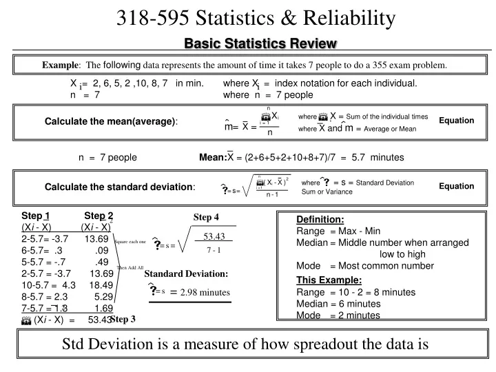
1. n X S i i = 1 m = = X n n 2 S ( X - X ) i s i = 1 = s = n - 1 Basic Statistics Review Example: The following data represents the amount of time it takes 7 people to do a 355 exam problem. X = 2, 6, 5, 2 ,10, 8, 7 in min. n = 7 where X = index notation for each individual. where n = 7 people i i whereS X = Sum of the individual times where X and m = Average or Mean Calculate the mean(average): Equation i n = 7 people Mean:X = (2+6+5+2+10+8+7)/7 = 5.7 minutes where s = s = Standard Deviation Sum or Variance Calculate the standard deviation: Equation Step 1 Step 2 (Xi - X) (Xi - X) 2-5.7= -3.7 13.69 6-5.7= .3 .09 5-5.7 = -.7 .49 2-5.7 = -3.7 13.69 10-5.7 = 4.3 18.49 8-5.7 = 2.3 5.29 7-5.7 = 1.3 1.69 S(Xi - X) = 53.43 Step 4 Definition: Range = Max - Min Median = Middle number when arranged low to high Mode = Most common number This Example: Range = 10 - 2 = 8 minutes Median = 6 minutes Mode = 2 minutes 2 53.43 Square each one Then Add All s = s = 7 - 1 Standard Deviation: = 2.98 minutes s = s 2 Step 3 Std Deviation is a measure of how spreadout the data is

2. 25 22 20 18 15 12 10 8 5 2 0 1.238 1.240 1.242 1.244 Bar Chart or Histogram Provides a visual display of data distribution Shape of Distribution May be Key to Issues • Normal (Bell Shaped) • Uniform (Flat) • Bimodal (Mix of 2 Normal Distributions) • Skewed left or right • Total number of bins is flexible but usually no more than 10 • By using an infinite number of bins, resultant curve is a distribution • Use T-Test to Compare Means, F-Test to Compare Variances

3. Target Specification Limit Histogram Specification Some Chance of Failure 1s 3s = z 66807ppm  The higher the number (Z) in front of the sigma symbol the lower the chance of producing a defect Much Less Chance of Failure 1s 3.4ppm 6s = z

4. Target Specification Limit Sigma vs Specification Some Chance of Failure 1s 3s = z 66807ppm  The higher the number (Z) in front of the sigma symbol the lower the chance of producing a defect Much Less Chance of Failure 1s 3.4ppm 6s = z

5. (with ± 1.5  shift) PPM 1,000,000 IRS - Tax Advice (phone-in) (140,000 PPM) Restaurant Bills 100,000 Doctor Prescription Writing Payroll Processing 10,000 • Average Company Airline Baggage Handling 1,000 100 10 Best-in-Class 1 6 2 3 4 5 7 Domestic Airline Flight Fatality Rate (0.43 PPM) Examples of Fault/Failure Rates on The Sigma Scale

6. MANUFACTURABILITY ASPECT Critical Measurement in Production: The desired state reality.... Unless you designed for it

7. Shift and Drift Inherent Capability of the Process Over time, a “typical” process will shift and drift by ~ 1.5 . . . also called “short-term capability” . . . reflects ‘within group’ variation Time 1 Time 2 Time 3 Time 4 Sustained Capability of the Process . . . also called “long-term capability” . . . reflects ‘total process’ variation LSL T USL Two Challenges: Center the Process and Eliminate Variation!

8. Other Methods to Present/Analyze Data

9. Linear Correlation of Input to Output 1.4 1.2 1 0.8 mArms 0.6 Vrms 0.4 Output 0.2 0 0 0.5 1 1.5 Input Plot or Scatter Plot Used to Illustrate Correlation or Relationships

10. Pareto Chart Root Cause Failures Example Used to Illustrate Contributions of Multiple Sources Excellent when data is abundant

11. Fishbone Diagram Ambient Temp Load Res Line Voltage Effect: Temp Of Amp For example Line Frequency Volume Input Amplitude Illustrates Cause & Effect Relationship

12. Year to Date Summary Replacement Parts Example

13. Intro to Reliability Evaluation • Basic Series Reli Method of an Electronic System: Component 1 l1 Component 2 l2 Component i li Component N lN • Each component has an associated reliability l • The System Reli lss is the sum of all the component l • lss = Sli • Reli l is expressed in “FITs” failure units • x FIT = x Failures/109 hours • Note: 109 hours = 1 Billion Hours

14. Definitions • lFIT = Failures per 109 hours lMTBF = 1/MTBF = 1/Mean time between failure in hours MTBF (years) = 1x109 / (lFIT * 8766 hours /year ) • R(t) = (Reliability at Time t) = Probability that a system will not fail for a time period “t,” assuming constant failure rate, R(t) = e-lt, Note: lMTBF in hr-1 and t in hr • Bathtub curve- typical reliability vs. time behavior

15. Example • An electronics assembly product has an MTBF of 20000 hours; constant failure rate • What is the probability that a given unit will work continuously for one year? • Reliability R(t) = e-lt • l = 1/MTBF = 1/20000 hr • l = 0.00005 hr-1 (Failure rate) • t = 8766 hours (1 year) • R(1yr) =e-(8766/20,000 = 0.65 = 65% • In other words, the Mean Time Between failures is 20,000 hours or about 2.3 years • but 35% of the units would likely fail in the first year of operation.

16. Example • An electronics product team has a goal of warranty cost which requires that a • Minimum reliability after 1 year be 99% or higher, R(1yr) >= 0.99 • What MTBF should the team work towards to meet the goal? Equations: R = e -lt and MTBF = 1/l Solve for MTBF: MTBF = 1/ l = 1/ {(-1/t) * ln R }, R = 0.99, t = 8766 hrs MTBF >= 872,000 hours (99.5 yrs) !

17. Some Typical Stresses • Environmental: Temp, Humid, Pressure, Wind, Sun, Rain • Mechanical: Shock, Vibration, Rotation, Abrasion • Electrical: Power Cycle, Voltage Tolerance, Load, Noise • ElectroMagnetic: ESD, E-Field, B-Field, Power Loss • Radiation: Xray (non-ionizing), Gamma Ray (ionizing) • Biological: Mold, Algae, Bacteria, Dust • Chemical: Alchohol, Ph, TSP, Ionic

18. Intro to Reliability Evaluation • Each l may be impacted by other factors or stresses, p: • Some commonly used factors • pT = Temperature Stress Factor • pV = Electrical Stress Factor • pE = Environmental Factor • pQ = Quality Factor • Overall Component l = lB * pT * pV * pE * pQ Where lB = Base Failure Rate for Component

19. Reliability Prediction Methods/Standards • Bellcore (TR-TSY-000332): • Developed by Bell Communications Research for general use in electronics industry although geared to telecom. • Highest Stress Factor is Electrical Stress • Data based upon field results, lab testing, analysis, device mfg data and US Military Std 217 • Stress Factors include environment, quality, electrical, thermal • US Military Handbook 217E: • Developed by the US Department of Defense as well as other agencies for use by electronic manufacturers supplying to the military • Describes both a “parts count” method as well as a “parts stress” method • Data is based upon lab testing including highly accelerated life testing (HALT) or highly accelerated stress testing (HAST) • Stress factors include environment and quality

20. Reliability Prediction Methods/Standards • HRD4 (Hdbk of Reliability Data for Comp, Issue 4): • Developed by the British Telecom Materials and Components Center for use by designers and manufacturers of telecom equipment • Stress factors include thermal as well as environment, quality with quality being dominant • Standard describes generic failure rates based upon a 60% confidence interval around data collected via telecom equipment field performance in the UK • CNET: • Developed by the French National Center of Telecommunications • Similar to HRD4, stress factors include thermal as well as environment and dominant quality • Data is based upon field experience of French commercial and military telecom equipment

21. Reliability Prediction Methods/Standards • Siemens AG (SN29500): • Developed by Siemens for internal uniform reliability predictions • Stress factors include thermal and electrical however thermal dominates • Standard describes failures rates based upon applications data, lab testing as well as US Mil Std 217 • Components are classified into technology groups each with tuned reliability model

22. Reliability Prediction • Basic Series Reli Method of an Electronic System: Component 1 l1 Component 2 l2 Component i li Component N lN • Above Reliability Prediction Model is flawed because; • Components may not have constant reliability rates l • lss = Sli • Component applications, stresses, etc may not be well matched by the method used to model reliability • Not all component failures may lead to a system failure • Example: A bypass capacitor fails as an open circuit

23. 595 Standard Failure Rates in FIT (Data is not accurate in all cases)

24. 595 Standard Stress Factors • Factor Definitions (may not represent standard models) • pT = Temperature Stress Factor = e[Ta/(Tr-Ta)] – 0.4 • Where Ta = Actual Max Operating Temp, Tr = Rated Max Op Temp, Tr>Ta • pV = Cap/Res/Transistor Electrical Stress Factor = e[(Va)/Vr-Va]-2.0 • Where Va = Actual Max Operating Voltage, Vr = Abs Max Rated Voltage, Vr>Va • pE = Environmental (Overall) Factor >>> • Indoor Stationary = 1.0 • Indoor Mobile = 1.5 • Outdoor Stationary = 2.0 • Outdoor Mobile = 2.5 • Automotive = 3.0 • pQ = Quality Factor (Parts and Assembly) • Mil Spec/Range Parts = 0.75 • 100 Hr Powered Burn In = 0.75 • Commercial Parts Mfg Direct = 1.0 • Commerical Parts Distributor = 1.25 • Hand Assembly Part = 3.0

25. Stress Factors Drive Simple: 595 Standard Deratings • Resistors, Potentiometers <= 50% maximum power • Caps/Res <= 60% maximum working voltage • Transistors <= 50% maximum working voltage • Note: Most discrete devices as well as linear IC’s have parameters which will vary with temperature which is expressed as Tc (temp coefficient). Typically a delta or percent of change per deg C from ambient.

26. MTBF Data Input Sheet for e-Reliability.com COST: $500 per report System / Equipment Name:Assembly Name:Quantity of this assembly:Parts List Number:Environment:Select One Of : GB, GF, GM, NS, NU, AIC, AIF, AUC, AUF, ARW, SF, MF, ML, or CLParts Quality:Select Either: Mil-Spec or Commercial/BellcoreQuantity Description---------- Bipolar Integrated Circuits IC / Bipolar, Digital 1-100 Gates IC / Bipolar, Digital 101-1000 Gates IC / Bipolar, Digital 1001-3000 Gates IC / Bipolar, Digital 3001-10000 Gates IC / Bipolar, Digital 10001-30000 Gates IC / Bipolar, Digital 30001-60000 Gates IC / Bipolar, Linear 1-100 Transistors IC / Bipolar, Linear 101-300 Transistors IC / Bipolar, Linear 301-1K Transistors IC / Bipolar, Linear 1001-10K Transistors, etc.  EXAMPLE: Actual Reli Tool Input List of components, their number, Environment conditions, components quality

27. Example Reliability calculation using actual MIL-HDBK-217F Failure rate of a Metal Oxide Semiconductor (MOS) can be expressed as Parameters are listed in MIL Data base. Temperature factor is modeled using Arrhenius type Eqn

28. Example Reliability report --------------------------------------------------------------------------------------- | | | | | Failure Rate in | | | | | | Parts Per Million Hours | | Description/ | Specification/ | Quantity | Quality |-------------------------| | Generic Part Type | Quality Level | | Factor | | | | | | | (Pi Q) | Generic | Total | | | | | | | | |=====================|================|==========|=========|============|============| | Integrated Circuit/ | Mil-M-38510/ | 16 | 1.00 | 0.07500 | 1.20000 | | Bipolar, Digital | B | | | | | | 30001-60000 Gates | | | | | | | | | | | | | | Integrated Circuit/ | Mil-M-38510/ | 8 | 1.00 | 0.01700 | 0.13600 | | Bipolar, Linear | B | | | | | | 101-300 Transistors | | | | | | | | | | | | | | Diode/ | Mil-S-19500/ | 2 | 2.40 | 0.00047 | 0.00226 | | Switching | JAN | | | | | | | | | | | | | | | | | | | | Diode/ | Mil-S-19500/ | 4 | 2.40 | 0.00160 | 0.01536 | | Voltage Ref./Reg. | JAN | | | | | | (Avalanche & Zener) | | | | | | | | | | | | | | Transistor/ | Mil-S-19500/ | 4 | 2.40 | 0.00007 | 0.00067 | | NPN/PNP | JAN | | | |

29. Reliability Prediction Drawbacks • Prediction Methods not always effective in representing future reality of a product. Tend to be pessimistic • Best utilized for design comparison, only if the same method is used • Single Stress Factors must be employed to represent a composite average or worst case of the population. Difficult to predict average stress levels, peak stress levels • Methods give an overall average failure rate, one dimensional • Time to failure distributions (Weibull) are two dimensional describing infantile failures as well as end of life failures

30. Reliability Growth Methods: HALT • HALT Strategy: Highly Accelerated Life Testing • One or more stresses used at accelerated amplitudes from what the product would see during application • Stress level is gradually increased until failure is detected • Failure is then autopsied to fundamental root cause • Corrective/Preventive action taken to remove chance of recurring failure • Test is then restarted • Must be prepared to destroy prototypes • Failure must be detectable, identifiable

31. Example of Accelerated Life Test (595 Team Project): “Rotating Bicycle Apparatus” Potential reliability stress is the periodic g-load (start-stop cycles). This causes fatigue failure mode (cracks in ceramic material, creep of plastics, adhesives, solder electrical contacts failure). • Estimation of the test protocol, plan and execution time. • The start-stop requirements for cycle: • 12 s to accelerate from 0 to 5 rev/sec max rotational speed (60 mph) • 5 s to decelerate from 5 rev/sec to 0. • 35 starts-stops cycles per day • One cycle time (from start to stop) is going to be: T = 12+5+5=20s, • where 5 s is added as a lag time to accommodate the transition from stopping back to starting Assuming the throughput 35 start-stops/day for 365 days/year the total number of rotation cycles for 1 year is 35*365=12775 cycles /year (=12775 start-stops). Assuming 20% overhead the total number of cycles is going to be 1.2*12775=15330 cycles/year. Test time worth of 1 year of the number of cycles is going to be 15330*20/(3600*24)=3.5 days

32. Reliability Growth Methods: HAST • HAST Strategy: Highly Accelerated Stress Testing • One or more stresses used at accelerated amplitudes from what the product would see during application • Stress level is constant, time to failure is primary measurement • Failure may also be autopsied to fundamental root cause • Corrective/Preventive action NOT necessarily taken • Test is then restarted using higher or lower stress amplitude to get additional data points • Used to find empirical relationship between stress level and time to failure (life)

33. Reliability Growth Methods: HASS • HASS Strategy: Highly Accelerated Stress Screening • Used in production to accelerate infantile failures and keep them from shipping to customers • Must have HAST data to understand how much life is expended with stress screen • One or more stresses used at slightly accelerated amplitudes from what the product would see during application • Common application is powered burn-in time during which electronics are powered and thermal cycled. (Example MIL-STD-883) Assemblies tested during or after burn-in for failure inducements

34. LFailures/Time infant mortality constant failure rate wearout Time Reliability Bathtub Curve • Infant mortality- often due to manufacturing defects ….. Can be screened out • In electronics systems, prediction models assume constant failure rates • (Bellcore model, MIL-HDBK-217F, others) • Understanding wearout requires knowledge of the particular device failure physics • - Semiconductor devices should not show wearout except at long times • - Discrete devices which wearout: Relays, EL caps, fans, connectors, solder

35. Causes of Electronic Systems Failure Reliability ofElectronic Circuits • Failures can generally be divided between intrinsic or extrinsic failures • Intrinsic failures- Inherent in the component technology • Electromigration (semiconductors, substrates) • Contact wear (relays, connectors, etc) • Contamination effects- e.g. channeling, corrosion, leakage • CTE mismatch and other Interconnection joint fatigue • Extrinsic failures- External stress to the components • ESD or Electrostatic discharge energy • Electrical overstress (over voltage, overload, overheat) • Shock (Sudden Mechanical Impact) • Vibration (Periodic Mechanical G force) • Humidity or condensable water • Package Mishandling, Bending, Shear, Tensile • Many “random” and infantile failures of components are due to extrinsic factors • Wearout failures are usually due to intrinsic failures

36. Physics of Failure: Accumulated Fatigue Damage (AFD) is related to the number of stress cycles N, and mechanical stress, S, using Miner’s rule Exponent Bcomes from the S-N diagram. It is typically between 6 and 25 Example: Solder Joint Shear Force voids Effective cross-sectional Area: D/2 Effective cross-sectional Area: D F Applied stress: Applied stress: Let  = 10, then AFD with voids will “age” about 1000x faster than AFD with no voids Voids in solder joints

37. a = N cycles D b T Failure Mechanism/Material b 316 Stainless Steel 1.5 4340 Steel 1.8 Solder (97Pb/03Sn) T > 30°C 1.9 Solder (37Pb/63Sn) T < 30°C 1.2 Solder (37Pb/63Sn) T > 30°C 2.7 General Failure Mechanism b Solder (37Pb/03Ag & 91Sn/09Zn) 2.4 Ductile Metal Fatigue 1 to 2 Aluminum Wire Bond 3.5 Commonly Used IC Metal Alloys and Au Al fracture in wire bonds 4.0 3 to 5 4 Intermetallics PQFP Delamination / Bond Failure 4.2 Brittle Fracture 6 to 8 ASTM 2024 Aluminum Alloy 4.2 Copper 5.0 Au Wire Bond Heel Crack 5.1 ASTM 6061 Aluminum Alloy 6.7 Alumina Fracture 5.5 Interlayer Dielectric Cracking 4.8-6.2 Silicon Fracture 5.5 Silicon Fracture (cratering) 7.1 Thin Film Cracking 8.4 Physics of failure: Thermal Fatigue Models Coefficients for Coffin - Manson Mechanical Fatigue Model • The Coffin - Manson model is most often used to model mechanical failures caused by thermal cycling in mechanical parts or electronics. (Most electronic failures are mechanical in nature) N cycles = number of cycles to failure at reference condition b = typical value for a given failure mechanism, a = prop constant • The values of the coefficient b for various failure mechanisms and materials (derived or taken from empirical data) Reference: “EIA Engineering Bulletin: Acceleration Factors”, SSB 1.003, Electronics - Industries Alliance, Government Electronics andInformation Technology Association Engineering Department, 1999.

38. a = N cycles D b T Normal operating conditions cycling 15C to 60C (T=45C) Plan for N Stress (Accelerated) cycles –40 to 125 C (T=165C) Find Mean life at stress level MTTF=4570 hrs=0.5 yrs Calculated acceleration factor and MTTF (and B10) @ normal stress: AF = Nuse / Nstress = (DT/DT)b = (165/45)2.7 = 33.4 MTTF (use)=MTTF(stress)*AF = 4570*33.4 = 152638hrs = 17.4 yrs

39. Appendices

40. b - ( ) t / h F(t) = 1 - e Reliability Distributions are non-Normal, require 2 parameters beta, b - slope/shape parameter Intro: Weibull Distribution ln ln (1 / (1 – F(t))) = b ln(t) – b ln(h) F(t) = Cumulative fraction of parts that have failed at time t Y = b X + a eta, h – characteristic life or scale parameter when t = h F(t) = 63.2% Knowing the distribution Function allows to address the following problem (anticipated future failure): What is the probability, P , that the failure will occur for the period of time T if it did not occur yet for the period of time t ? (T>t) P={F(T)-F(t)}/[1-F(t)]=

41. Physical Significance of Weibull Parameters When Weibull distribution parameters are defined, B10 and MTTF can be computed. 99 MTTF = mean time to failure (non-repairable) = h G ( 1 + 1/b ) When b = 1.0, MTTF = h When b = 0.5, MTTF = 2h Cumulative Failure (%) F(t) MTBF = mean time between failure (repairable) (MTBSC) b Slope = = total time on all systems / # of failures 10 When there is no suspension data, MTBF = MTTF B10 100 1 10 Time to Failure (t) The slope parameter, Beta (b), indicates failure type b < 1 rate of failure is decreasing infantile (early) failure b = 1 rate of failure is constant random failure b > 1 rate of failure is increasing wear out failure

42. Estimating Reliability from Test Data • In testing electronics assemblies or parts, there are frequently few (or no) failures • How do you estimate the reliability in this case? • Use the chi-squared distribution and the following equation: • MTBF = 2 * Number of hours on test * Acceleration factor / c2 • In this equation, c2 is a function of two variables • n, the degrees of freedom, defined as n= 2 * number of failures + 2 • and F, the confidence level of the results (e.g. 90%, 95%, 99%)

43. Example • The following test was conducted: • A new design was qualified by testing 20 boards for 1000 hours • The test was conducted at elevated temperatures, where the test would accelerate • failures by 10X the usage rate • One board failed at 500 hours, the other 19 passed for the full 1000 hours • What is the MTBF of the board design at 90% confidence? • Solution: • First, determine n = 2 * number of failure + 2 = 4; so c2 = 7.78 (at 90% confidence) • Second, determine number of hours = 19 samples * 1000 + 1 * 500 = 19, 500 hours • So, the answer is: • MTBF = 2 * 19500 (total hours) * 10 (acceleration factor) / 7.78 = 50, 128 hours

44. The calculations are based on the Binomial Distribution and the following formula: where: n = sample size p = proportion defective r = number defective Confidence Level CL =  = probability of k or fewer failures occurring in a test of n units Pass/Fail Test Sample Sizes? Example: Suppose that 3 failed parts have been observed in the test equivalent to 1 year life, what minimum sample size is needed to be 95% confident that the product is no more than 10% defective? Inputs in the formula are: p =0.1(10%), r = 3, CL = 0.95(95%), P(r<k) = 0.05 and calculate n. The minimum sample size will be 76. Reliability test should start using just a few parts in order to get preliminary number of failed parts. Using this data a required sample size can then be estimated.

45. MTTF~=10 years (B10=1 year) results in failure rate 1-F=1-exp(-1/10*10)=0.63, i.e. 63% of units on average will fail for 10 years MTTF= 47.5 years (B10=5 years) results in failure rate 1-F=1-exp(-1/47.5*10)=0.19, i.e. 19% of units on average will fail for 10 years. System Reliability Target Must be Allocated