Download
1 / 19
190 likes | 388 Views
Basic Probability - Part 2. Kwang In Kim A. I. Lab. Contents. Expectation, variance of RVs Conditional probability Independence Joint probability and marginalization. Random Variables. Suppose a probability P is defined on S

E N D
Basic Probability - Part 2 Kwang In Kim A. I. Lab
Contents • Expectation, variance of RVs • Conditional probability • Independence • Joint probability and marginalization
Random Variables • Suppose a probability P is defined on S • Sometimes we are interested in defining a function X from S to another space N and doing probabilistic reasoning in N • In this case, probability on N can be induced from that of S • E.g., when you toss three coins you might be interested in only the number of heads (rather than exact outcome) • S: {HHH, HHT, HTH, HTT, THH, THT, TTH, TTT} • N: {0,1,2,3} • X:SNsummarizes events in S • Probability of X=2 can be induced from P:P(X-1(2))=P ({HHT,HTH,THH})=3/8 • Such function X is called a random variable (RV)
Random Variables (Cont’d) • Suppose a probability P is defined on S • For a function X:SN to be a RV it should induce a probability G on N based on P: • For each event BN, X-1(B)S and X-1(BC)S • For events B,C N,X-1(BC)S, etc. • Inverse image of σ-algebra on N should be included in the σ-algebra on S • Probability distribution functions can be induced in N • In practice, virtually any function you can think of satisfies this condition • Often, output space (or sample space) N is • R: X is called a random variable • RN: X is called a random vector • R: X is called a random process • A random vector and a random process can be regarded as a collection of random variables • When N is • Finite or countable: X is called a discrete RV • Uncountable: X is called a continuous RV
Expectation / Variance of RVs • It would be useful if we summarize essential properties of RVs • Expectation • Weighted average of possible events; each value of event weighted by probability • Limit of average (c.f., probability: limit of relative frequency) • Center of gravity of mass distribution • For discrete case • E[X]={x:p(X=x)>0} xp(X=x), p: probability mass function • For continuous case • E[X]=xf(X=x)dx, f: probability density function • Varince • Variation or spread of events • Mean of squared distance from expectation • Moment of inertia (mechanics) • Var[X] =E[(X-E[X])2]=E[X2]–(E[X])2 • Standard deviation: (Var[X])
Examples • Suppose X denote outcome when you roll a fair (uniform) die • Sample space S=N={1,2,3,4,5,6}* • p(1)=p(2)=p(3)=p(4)=p(5)=p(6)=1/6 • E[X]={p(x)>0}xp(x)#=i=1,…,6ip(i)=7/2 • (E[X])2={p(x)>0}x2p(x)=i=1,…,6(i)2p(i)=91/6 • Var[X]= E[X2]–(E[X])2=91/6-(7/2)2=35/12 • Var[X]1.71 * X is identity function here# event X=x is denoted simply as x
Examples • Suppose density function of X is given asf(x)=2x if 0x1=0 otherwise • Then • E[X]= xf(x)dx = 2x2dx=2/3 • E[X2]= x2f(x)dx = 2x3dx=1/2 • Var[X]= E[X2]–(E[X])2=1/2-(2/3)2=1/18 • Var[X]0.24
Conditional Probability • We are interested in calculating probabilities when partial information concerning result of experiment is available • E.g., tossing 3 coins • What is probability of at least two H? • You may count all possible 8 cases and find that HHH,HHT,HTH,THH satisfy condition • Probability: 1/2 • You observed that first coin showed H; Then, what is probability of at least two H? • You may count all possible 4 cases of remaining two coins and find HH,HT,TH satisfy condition • Probability: ¾ • Probability influenced by information
Conditional Probability (Cont’d) • In probability language, previous example states “conditional probability of at least two H given first one H is 3/4”orP(“at least two H”|”first one H”)=3/4 or P(A|B)=3/4 whereA=“at least two H” and B=”first one H” • Cf., probability of joint occurrence of events are called joint probability AB={HHH, HHT, HTH} with P(AB)=3/8 • Joint occurrence of A and B can be regarded as new event AB • Corresponding RV is called joint RV • Details will be given later
Calculating Conditional Probability • Conditional probability of an event given another event • A new probability valueP(A|B) is induced based on probabilities of events B and AB, such that If P(B)>0,P(A|B)=P(AB)/P(B) • Conditional probability of RV given another event • A new probability functionP(X|B) is induced from P(B) and P(XB) such that If P(B)>0,P(X|B)=P(XB)/P(B) or If P(B)>0,P(Ai|B)=P(AiB)/P(B) where Ai are all possible events ofX
Calculating Conditional Probability (Cont’d) • Conditional probability of RV given another RV • In general, a set of new probability functionsP(X|Y) is induced based on two RVs Y and XY such that If P(Y)>0,P(X|Y)=P(XY)/P(Y) or If P(Bi)>0,P(X|Bi)=P(XBi)/P(Bi) where Bi are all events ofY • E.g., in coin tossing example you may defineX=number of total head Y=face of first coin, then • P(“at least two H”|”first one H”)=P(X2|Y=H)=3/4 • P(“only one H”|”first one H”)=P(X=1|Y=H)=1/4, etc. • For each value y of YP(X|y) defines a probability; Therefore it satisfies probability axioms
Independence • Not every information affects our knowledge on a given problem • E.g., You toss two coins, and let’s denote • A = first coin shows H • B = second coin shows H • then, P(A)=½ and P(A|B)=½ • Two events A and B are independent if knowing one event does not affect probability of the otherP(A)=P(A|B) • In general two RVs X and Y are independent if P(Ai)=P(Ai|Bi) for all possible events Ai and Bi of X and Y, respectively P(X)=P(X|Y) • E.g., X and Y are independent when they denote faces of two coins • Alternative definition: X and Y are independent ifP(XY)=P(X)P(Y)(P(X|Y)=P(XY)/P(Y) P(X|Y)P(Y) =P(XY) P(X)P(Y) =P(XY)) Cf., Bayes’ formula: P(X|Y)=P(Y|X)P(X)/P(Y) • Independence implies • p(X)p(Y) =p(XY) where p is mass function for discrete RV • f(X)f(Y) =f(XY) where f is pdf for continuous RV
Independence • Three RVs X, Y, and Z are (mutually) independent if P(XYZ)=P(X)P(Y)P(Z) • Warning, pair-wise independences P(XY)=P(X)P(Y), P(XZ)=P(X)P(Z), P(YZ)=P(Y)P(Z)do not imply mutual independence • E.g., suppose you have uniform probability ¼ for i=1,…,4 andX=1 if i=1 or 2, 0 otherwise,Y=1 if i=2 or 4, 0 otherwise,Z=1 if i=2 or 3, 0 otherwise, then • P(X=1,Y=1,Z=1)=1/4P(X=1)P(Y=1)P(Z=1)=1/8 • If (X=1,Y=1) occurs (Z=1) always occurs
Joint Probability Examples • Joint events • Tossing three coins; let • A: at least two H • B: first one H • AB: both A and B occur then • P(A) = ½ • |{HHH,HHT,HTH,THH}|/|{HHH,HHT,HTH,HTT,THH,THT,TTH,TTT}| • P(B) = ½ • |{H}|/|{H,T}|or |{HHH,HHT,HTH,HTT}|/|{HHH,HHT,HTH,HTT,THH,THT,TTH,TTT}| • P(AB)=3/8 • |{HHH,HHT,HTH}|/|{HHH,HHT,HTH,HTT,THH,THT,TTH,TTT}| • Joint RVs • X=number of total head (P(A)=P(X>2)) • Y=face of first coin, then (P(B)=P(Y=H)) • XY=number of total head and face of first coin (P(AB)=P(X>2,Y=H))
Joint Probability • In general, joint probability of two RVs is different from product of probabilities of individual RV • E.g., probability mass functions of coin tossing example are • P(X): P(X=0), P(X=1), P(X=2), P(X=3) (4 entries) • P(Y): P(Y=H), P(Y=T) (2 entries) • P(XY): P(X=0, Y=H), P(X=0, Y=T),P(X=1, Y=H), P(X=1, Y=T)P(X=2, Y=H), P(X=2, Y=T)P(X=3, Y=H), P(X=3, Y=T) (4x2 entries) • But it is possible to factorize a joint RV into two individual RVs
Marginalization • Suppose X and Y are discrete random variables and we know P(XY). ThenP(X=x)=P(X=x,YN) =P(XY{x}N) =P(XYj{(x,yj)}) =jP(x,yj)where N={y1,…yN} is sample space of YThe last summation is called a marginalization of XY w.r.t. Y • E.g., coin tossing example
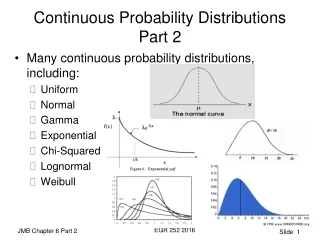
Marginalization for Continuous Random Variables • Suppose X and Y are continuous random variables and we know f(XY). Then for any event A for XP(XA)=P(XA and YN) =ANf(x,y)dxdy =ANf(x,y)dydx =Ag(x)dxwhere g(x)=Nf(x,y)dy and N is sample space of YThe last integral called a marginalization of XY w.r.t. Y
Complexity of Joint Probability • Suppose X1,…,Xn are all discrete RVs, with same sample space N of size N • Knowing probability for Xi • Knowing probability mass function for Xi • Knowing a table of size N • Therefore, knowing probabilities for each X1,…,Xn • Knowing a table of size nN • But sample space for X1,…,Xn is Nn whose size is Nn • Therefore, knowing joint probability for X1,…,Xn • Knowing a table of size Nn • Thus the joint probability contains much more information than all its marginalization together • For independent RVs, complexity of joint probability reduces to that of marginal
References • Part of this slide comes from Dr. Jahwan Kim’s Lecture slide “Probability” • Introductory textbook • S. Ross, A first course in probability, 6th ed. • Textbooks for measure theoretic probability • P. Billingsley, Probability and Measure, 3rd ed. • D. Pollard, User’s Guide to Measure Theoretic Probability • Reference book • E. Jaynes, Probability Theory: The Logic of Science