Download

1 / 33
340 likes | 474 Views
Values & means (Falconer & Mackay: chapter 7). Sanja Franic VU University Amsterdam 2011. Intro:

E N D
Values & means(Falconer & Mackay: chapter 7) Sanja Franic VU University Amsterdam 2011
Intro: As discussed in previous class, the genetic properties of a population are expressible in terms of gene frequencies and genotype frequencies. To deduce the connection between these, on the one hand, and the quantitative differences in a measured characteristic, on the other, we introduce the concept of value. This value is expressible in the metric units in which the character is measured. To denote the value observed upon measuring a trait, we will use the term phenotypic value (e.g., height in cm).
The measured value of a trait, or its phenotypic value (P), is typically conceptualized as a sum of two components, one attributable to the particular assemblage of segregating genes relevant to the phenotype in question (the genotypic value, G), and the other to all of the non-genetic factors affecting the phenotype (environmental deviation, E): • The mean environmental deviation in the population is typically scaled at zero; thus the mean phenotypic value equals the mean genotypic value (μP = μG). * • * Note: Here we refer only to the component of P that varies in the population; thus the effects of monomorphic genes (i.e., genes with only one allele present in the population), as well as the non-variable aspects of the environment, are ignored (but may be modeled by addition of appropriate constants). P = G + E Phenotypic value Genotypic value Environmental deviation
For the purposes of deduction, we assign arbitrary genotypic values to genotypes: Consider, for instance, a single locus with two alleles, A1 and A2. The genotypic values of the two homozygotes (A1A1 and A2A2) and that of the heterozygote (A1A2) may be denoted +a, -a, and d, respectively. The point of zero genotypic value is defined as the midpoint between the two homozygotes. The value of d reflects the degree of genetic dominance: in the absence of dominance, d = 0; if A1 is dominant over A2, d > 0; if A2 is dominant over A1, d < 0; in case of overdominance, d > a or d < -a. A2A2 A1A2 A1A1 Genotype Genotypicvalue - a 0 d + a Genotype frequency q2 2pq p2
How do gene frequenciesinfluence the mean of the character in the population? • If the relative frequencies with which the A1 and A2 alleles occur in the population of interest are denoted p and q, respectively (p + q = 1), the frequencies of the genotypes arising from the process of random mating between individuals within this population are given by the binomial expansion (p + q)2 = p2 + 2pq + q2: • The mean genotypic value of this locus may be obtained by multiplying the value of each genotype by its frequency and summing over the three genotypes.
How do gene frequenciesinfluence the mean of the character in the population? • If the relative frequencies with which the A1 and A2 alleles occur in the population of interest are denoted p and q, respectively (p + q = 1), the frequencies of the genotypes arising from the process of random mating between individuals within this population are given by the binomial expansion (p + q)2 = p2 + 2pq + q2: • The mean genotypic value of this locus may be obtained by multiplying the value of each genotype by its frequency and summing over the three genotypes. A2A2 A1A2 A1A1 Genotype Genotypicvalue - a 0 d + a Genotype frequency q2 2pq p2
How do gene frequenciesinfluence the mean of the character in the population? • If the relative frequencies with which the A1 and A2 alleles occur in the population of interest are denoted p and q, respectively (p + q = 1), the frequencies of the genotypes arising from the process of random mating between individuals within this population are given by the binomial expansion (p + q)2 = p2 + 2pq + q2: • The mean genotypic value of this locus may be obtained by multiplying the value of each genotype by its frequency and summing over the three genotypes: μG = p2a + 2pqd - q2a = a(p – q)(p + q) + 2dpq = a(p – q) + 2dpq. A2A2 A1A2 A1A1 Genotype Genotypicvalue - a 0 d + a Genotype frequency q2 2pq p2
μG = μP = a(p – q) + 2dpq • If there is no dominance (d=0), the mean is proportional to the gene frequency: • If there is complete dominance (d=a), how can we express the mean (in terms of a and q)? • Thus the mean is in this case proportional to the square of gene frequency. • The total range of values attributable to a locus, in the absence of overdominance, is 2a (i.e., if only A1 were present in the population [p=1], the mean would equal a; if only A2 were present [q=1], it would equal –a). Term attributable to homozygotes Term attributable to heterozygotes
μG = μP = a(p – q) + 2dpq • If there is no dominance (d=0), the mean is proportional to the gene frequency: • μG = a(p – q) = a(1 – q – q) = a(1 – 2q). • If there is complete dominance (d=a), how can we express the mean (in terms of a and q)? • Thus the mean is in this case proportional to the square of gene frequency. • The total range of values attributable to a locus, in the absence of overdominance, is 2a (i.e., if only A1 were present in the population [p=1], the mean would equal a; if only A2 were present [q=1], it would equal –a). Term attributable to homozygotes Term attributable to heterozygotes
μG = μP = a(p – q) + 2dpq • If there is no dominance (d=0), the mean is proportional to the gene frequency: • μG = a(p – q) = a(1 – q – q) = a(1 – 2q). • If there is complete dominance (d=a), how can we express the mean (in terms of a and q)? • μG = a(p – q) + 2apq = a(1 – 2q) + 2aq(1 – q) • = a(1 – 2q) + 2aq + 2aq2 • = a(1 – 2q + 2q + 2q2) • = a(1 – 2q2). • Thus the mean is in this case proportional to the square of gene frequency. • The total range of values attributable to a locus, in the absence of overdominance, is 2a (i.e., if only A1 were present in the population [p=1], the mean would equal a; if only A2 were present [q=1], it would equal –a). Term attributable to homozygotes Term attributable to heterozygotes
Because genotypic values a and d are defined as deviations from the midpoint between the two homozygotes: • the population mean μGis a deviation from the mid-homozygote value, which is the zero point of the scale. Expressing the mean as a deviation from some other value is possible by addition or subtraction of appropriate constants. A2A2 A1A2 A1A1 Genotype Genotypicvalue - a 0 d + a Genotype frequency q2 2pq p2
Average effect In deducing the properties of a population connected with its family structure, one must deal with transmittion of value from parent to offspring. This cannot be done by means of genotypic values alone, as parents pass on their genes and not their genotypes to offspring (i.e., each of the two alleles at a locus is inherited from one of the parents). The allelic equivalent of the genotypic value is average effect of the allele. The average effect of an allele is the mean deviation from the population mean of individuals who received that allele from one parent, the other allele having come at random from the population. In other words, if a number of gametes all carrying A1 unite at random with gametes from the population, the mean of the genotypes so produced deviates from the population mean by an amount which is the average effect of the A1 allele.
For instance: if a number of gametes carrying the A1 allele unite at random with gametes from the population (where p is the frequency of the A1 allele and q of the A2 allele), the frequencies of the genotypes produced will be ...? Taking into account these frequencies and the genotypic values associated with each genotype, the mean genotypic value of the locus may be expressed as: pa + qd. Subtracting the population mean from this expression yields the expression for the average effect of the A1 allele: α1 = pa + qd - μG= pa + qd – [a(p – q) + 2dpq] = q[a + d(q – p)]. Correspondingly, the average effect of A2 is α2 = – p[a + d(q – p)].
For instance: if a number of gametes carrying the A1 allele unite at random with gametes from the population (where p is the frequency of the A1 allele and q of the A2 allele), the frequencies of the genotypes produced will be p of A1A1 and q of A1A2. Taking into account these frequencies and the genotypic values associated with each genotype, the mean genotypic value of the locus may be expressed as: pa + qd. Subtracting the population mean from this expression yields the expression for the average effect of the A1 allele: α1 = pa + qd - μG= pa + qd – [a(p – q) + 2dpq] = q[a + d(q – p)]. Correspondingly, the average effect of A2 is α2 = – p[a + d(q – p)].
The average effect may also be expressed in terms of the average effect of gene substitution, which is simply the difference between the average effects of the two alleles: α = α1 – α2 = ...? The average effects of the two alleles may be conveyed in terms of the average effect of gene substitution: α1 = α + α2 =a + d(q – p) – p[a + d(q – p)] = (1 – p) [a + d(q – p)] = qα. Similarly, it can be shown that α2 = -pα.
The average effect may also be expressed in terms of the average effect of gene substitution, which is simply the difference between the average effects of the two alleles: α = α1 – α2 = a + d(q – p). The average effects of the two alleles may be conveyed in terms of the average effect of gene substitution: α1 = α + α2 =a + d(q – p) – p[a + d(q – p)] = (1 – p) [a + d(q – p)] = qα. Similarly, it can be shown that α2 = -pα.
Breeding value As mentioned, parents pass on their genes and not their genotypes to the progeny. Therefore the mean genotypic value of the progeny is determined by the average effects of the parents’ genes. The value of an individual, judged by the mean of its progeny, is termed the breeding value. If an individual is mated to a number of individuals taken from the population at random, then its breeding value is twice the deviation of the progeny from the population mean. The deviation is doubled because the parents in question provides only half of the genes in the progeny, the other half coming at random from the population. In terms of average effects, an individual’s breeding value for a single locus may be obtained by summing the average effects over the two alleles at the locus, thus:
In the absence of between-locus interaction (i.e., of non-additive combination of genotypic values across loci), extension to multiple loci is straightforward: the breeding value of a genotype is the sum of the breeding values attributable to each of the separate loci. The mean breeding value (in a population in H-W equilibrium) may be obtained by multiplying the breeding value of each genotype by that genotype’s frequency, and summing over the genotypes: The breeding value is also referred to as the additive genotype (A), and variation in breeding value ascribed to the ‘additive effects’ of genes (next lecture will address variation). The expected breeding value of any individual is the average of the breeding values of its two parents, and is equal to the individual’s expected phenotypic value. Different offspring of the same parents will differ in breeding value according to which allele they receive from each parent. Over a large number of progeny from the same parents, however, the expected breeding value is: AO = PO = ½ (Af + Am), where f and m denote father and mother, respectively.
In the absence of between-locus interaction (i.e., of non-additive combination of genotypic values across loci), extension to multiple loci is straightforward: the breeding value of a genotype is the sum of the breeding values attributable to each of the separate loci. The mean breeding value (in a population in H-W equilibrium) may be obtained by multiplying the breeding value of each genotype by that genotype’s frequency, and summing over the genotypes: The breeding value is also referred to as the additive genotype (A), and variation in breeding value ascribed to the ‘additive effects’ of genes (next lecture will address variation). The expected breeding value of any individual is the average of the breeding values of its two parents, and is equal to the individual’s expected phenotypic value. Different offspring of the same parents will differ in breeding value according to which allele they receive from each parent. Over a large number of progeny from the same parents the expected breeding value is: AO = PO = ½ (Af + Am), where f and m denote father and mother, respectively.
Dominance deviation The breeding value is the additive component of the genotypic value. The remainder of the genotypic value is termed the dominance deviation (D): Dominance deviations represent within-locus interactions, i.e. non-additive co-action of alleles within a locus. In other words, they account for the effects not accounted for by the additive effects of two alleles at a locus taken singly (if the joint effects of the 2 alleles at a locus does not equal the mean of their individual effects, then we talk about dominance deviations). P = G + E Phenotypic value Genotypic value Environmental deviation G = A + D Genotypic value Breeding value Dominance deviation
D may be obtained by subtracting the breeding value from the genotypic value (D = G – A). For this, we must first express the genotypic value of each genotype as a deviation from the population mean. E.g., the genotypic value of the genotype A1A1 equals a, thus expressed as a deviation from the population mean it is: a - [a(p – q) + 2dpq] = a – ap + aq – 2dpq = a(1 – p + q) – 2dpq = a(q + q) – 2dpq = 2aq – 2dpq = 2q(a – dp) Since a = α – d(q – p), the genotypic value above can also be expressed as 2q(α – dp). If we subtract the breeding value for this genotype (2qα) from the genotypic value (thus, if we apply D = G – A), we get the dominance deviation as -2q2d.
As can be seen from the table below, all the dominance deviations are functions of d. Thus in the absence of dominance (i.e., when d=0), breeding values and the genotypic values coincide (G=A). Genes that exhibit no dominance are often referred to as additive genes. Given that the mean breeding value and the mean genotypic value are equal (μP = μG, and μP = μA; thus μG = μA) and that the mean genotypic value is zero, as shown (thus μP = μG = μA = 0), it follows that the mean dominance deviation is zero (because μG = μA + μD, and μG = μA = 0). An alternative way to derive this is laid out in the table below.
As can be seen from the table below, all the dominance deviations are functions of d. Thus in the absence of dominance (i.e., when d=0), breeding values and the genotypic values coincide (G=A). Genes that exhibit no dominance are often referred to as additive genes. Given that the mean breeding value and the mean genotypic value are equal (μP = μG, and μP = μA; thus μG = μA) and that the mean genotypic value is zero, as shown (thus μP = μG = μA = 0), it follows that the mean dominance deviation is zero (because μG = μA + μD, and μG = μA = 0). An alternative way to derive this is laid out in the table below.
As can be seen from the table below, all the dominance deviations are functions of d. Thus in the absence of dominance (i.e., when d=0), breeding values and the genotypic values coincide (G=A). Genes that exhibit no dominance are often referred to as additive genes. Given that the mean breeding value and the mean genotypic value are equal (μP = μG, and μP = μA; thus μG = μA) and that the mean genotypic value is zero, as shown (thus μP = μG = μA = 0), it follows that the mean dominance deviation is zero (because μG = μA + μD, and μG = μA = 0). An alternative way to derive this is laid out in the table below.
P = G + E Phenotypic value Genotypic value Environmental deviation
Breeding value Dominance deviation P = G + E = A + D + E Phenotypic value Genotypic value Environmental deviation
Breeding value Dominance deviation P = G + E = A + D + E Phenotypic value Genotypic value Environmental deviation μP = μG + μE = μA + μD + μE
Breeding value Dominance deviation P = G + E = A + D + E Phenotypic value Genotypic value Environmental deviation μP = μG + μE = μA + μD + μE = 0 + 0 + 0
Graphical representation of G (closed circles) and A (open circles) for genotypes at a diallelic locus, where A1 and A2 appear at frequencies p and q, respectively. X-axis: number of A1 alleles in the genotype. Y-axis, left: scale of arbitrarily assigned genotypic values –a, d, and a. Y-axis, right: deviations from the population mean. In the figure d=3/4a, and q=1/4.
Graphical representation of G (closed circles) and A (open circles) for genotypes at a diallelic locus, where A1 and A2 appear at frequencies p and q, respectively. X-axis: number of A1 alleles in the genotype. Y-axis, left: scale of arbitrarily assigned genotypic values –a, d, and a. Y-axis, right: deviations from the population mean. In the figure d=3/4a, and q=1/4. α1+α2 2α1 - α1 – α2 = α1 – α2 = α 2α1
Interaction deviation If the genotypic value refers to an aggregate value of genotypes across more than one locus, the expression for G takes on the form: G = A + D + I, where I stands for interaction deviation arising from possible non-additive gene co-action across loci (i.e., epistasis). If the interaction deviation is zero, the genes across multiple loci are said to act additively (note: thus additivity may refer to two different things: within a locus it refers to the absence of dominance, whereas between loci it denotes the absence of epistasis). If values are expressed as deviations from the population mean, then the mean interaction deviation in the population is zero (because μG = μA + μD + μI , and μG = μA = μD = 0). Note: All of the population values discussed in the present lecture (mean genotypic value, average effect, mean breeding value, mean dominance deviation, and mean interaction deviation) depend not only on the geotypic values a and d, but also on the gene frequencies in the population (p and q). Thus all of these not only describe the genes concerned, but are also properties of the populations under study.
Homework: Assignments 7.1, 7.2, 7.5, and 7.6 Suzanne’squestion