Download

1 / 51
510 likes | 516 Views
Explore linear regression models of connectivity and structural equation modeling (SEM) in understanding the relationships between variables. Analyze connectivity patterns and examine modulatory effects. Compare nested models and assess goodness-of-fit using Chi-square statistics. Incorporate hemodynamic deconvolution for BOLD time series analysis.

E N D
Linear regression models of connectivity Structural equation modelling (SEM) z2 z1 b12 y2 y1 b13 b32 y3 z3 0 b12b13 y1 y2 y3 = y1 y2 y3 0 0 0 + z1 z2 z3 0 b320 y – time series b - path coefficients z – residuals (independent) • Minimises difference between observed and implied covariance structure • Limits on number of connections (only paths of interest) • No designed input - but modulatory effects can enter by including bilinear terms as in PPI
Linear regression models of connectivity Inference in SEM – comparing nested models • Different models are compared that either include or exclude a specific connection of interest • Goodness of fit compared between full and reduced model: - Chi2 – statistics • Example from attention to motion study: modulatory influence of PFC on V5 – PPC connections H0: b35 = 0
Modulatory interactions at BOLD versus neuronal level • HRF acts as low-pass filter • especially important in high frequency (event-related) designs • Facit: • either blocked designs or • hemodynamic deconvolution of BOLD time series – incorporated in SPM2 Gitelman et al. 2003
Basics Z2 Z4 Z5 Z1 Z2 Z3
Basics Z2 Z4 Z5 Z1 Z2 Z3 Latent (intrinsic) connectivities: a
Basics Z2 Z4 = a42z2 Z5 Z1 Z2 Z3 Latent (intrinsic) connectivities: a
Increase: Z = 1 - e (-t/r) r = time constant in [s] r = 1s t=1s Z = 1 - e-1 = 63% r = 2s t=1s Z = 1 - e-1/2 = 30% Short r fast increase Rate = 1/r in [1/s] or Hz Long rate fast increase ms
Basics Z2 ż4 = a42z2 Z5 Z1 Z2 Z3 Latent (intrinsic) connectivities: a
Basics Z2 ż4 = a42z2 + a45z5 Z5 Z1 Z2 Z3 Latent (intrinsic) connectivities: a
Basics Z2 ż4 = a42z2 + a45z5 ż5 = a53z3 +a54z4 Z1 ż2 = a21z1 +a23z3 ż3 = a35z5 Latent (intrinsic) connectivities: a
Basics Z2 ż4 = a44z4 + a42z2 + a45z5 ż5 = a53z3 +a54z4 Z1 ż2 = a21z1 +a23z3 ż3 = a35z5 Latent (intrinsic) connectivities: a
Basics Z2 ż4 = a44z4 + a42z2 + a45z5 ż5 = a55z5 +a53z3 +a54z4 ż2 = a22z2 + a21z1+a23z3 ż1 = a11z1 ż3 = a35z5 +a35z5 Latent (intrinsic) connectivities: a
Basics Z2 ż4 = a44z4 + a42z2 + a45z5 Stimuli u1 “perturbation” ż5 = a55z5 +a53z3 +a54z4 ż2 = a22z2 + a21z1+a23z3 ż1 = a11z1 ż3 = a35z5 +a35z5 Latent (intrinsic) connectivities: a
Basics Z2 ż4 = a44z4 + a42z2 + a45z5 Stimuli u1 “perturbation” ż5 = a55z5 +a53z3 +a54z4 ż2 = a22z2 + a21z1+a23z3 ż1 = a11z1 + c11u1 ż3 = a35z5 +a35z5 Latent (intrinsic) connectivities: a Extrinsic influences: c
Basics “context” Z2 ż4 = a44z4 + a42z2 + a45z5 Set u2 Stimuli u1 “perturbation” ż5 = a55z5 +a53z3 +a54z4 ż2 = a22z2 + a21z1+a23z3 ż1 = a11z1 + c11u1 ż3 = a35z5 +a35z5 Latent (intrinsic) connectivities: a Extrinsic influences: c
Basics “context” Z2 ż4 = a44z4 + a42z2 + a45z5 Set u2 Stimuli u1 “perturbation” ż5 = a55z5 +a53z3 +a54z4 ż2 = a22z2 + a21z1+a23z3 ż1 = a11z1 + c11u1 ż3 = a35z5 +a35z5 Latent (intrinsic) connectivities: a Extrinsic influences: c
Basics “context” Z2 ż4 = a44z4 + a42z2 + a45z5 Set u2 Stimuli u1 “perturbation” ż5 = a55z5 +a53z3 +a54z4 ż2 = a22z2 + a21z1+a23z3 ż1 = a11z1 + c11u1 ż3 = a35z5 +a35z5 Latent (intrinsic) connectivities: a Induced connectivities: b Extrinsic influences: c
Basics “context” Z2 ż4 = a44z4 + a42z2 + a45z5 Set u2 Stimuli u1 “perturbation” ż5 = a55z5 +a53z3 +a54z4 ż2 = a22z2 + a21z1 +(a23 + b23u2)z3 ż1 = a11z1 + c11u1 ż3 = a35z5 +a35z5 Latent (intrinsic) connectivities: a Induced connectivities: b Extrinsic influences: c
Basics “context” Z2 ż4 = a44z4 + (a42 + b42u2)z2 + a45z5 Set u2 Stimuli u1 “perturbation” ż5 = a55z5 +a53z3 +a54z4 ż2 = a22z2 + a21z1 +(a23 + b23u2)z3 ż1 = a11z1 + c11u1 ż3 = a35z5 +a35z5 Latent (intrinsic) connectivities: a Induced connectivities: b Extrinsic influences: c
bilinear Basics “context” Z2 ż4 = a44z4 + (a42 + b42u2)z2 + a45z5 Set u2 Stimuli u1 “perturbation” ż5 = a55z5 +a53z3 +a54z4 ż2 = a22z2 + a21z1 +(a23 + b23u2)z3 ż1 = a11z1 + c11u1 ż3 = a35z5 +a35z5 Latent (intrinsic) connectivities: a Induced connectivities: b Extrinsic influences: c
bilinear Basics “context” Z2 ż4 = a44z4 + (a42 + b42u2)z2 + a45z5 Set u2 Stimuli u1 “perturbation” ż5 = a55z5 +a53z3 +a54z4 ż2 = a22z2 + a21z1 +(a23 + b23u2)z3 ż1 = a11z1 + c11u1 ż3 = a35z5 +a35z5 Latent (intrinsic) connectivities: a Induced connectivities: b Extrinsic influences: c
Basics Neuron BOLD ?
Basics Neuron BOLD BOLD = f(z and 4 state variables) Hemodynamic model: 4 state variables: vasodilatory signal, flow, venous volume, dHb content
SPM{F} A2 A1 WA An example
Stimulus (perturbation), u1 Set (context), u2 A2 . A1 . WA
Stimulus (perturbation), u1 Set (context), u2 A2 . A1 . WA Full intrinsic connectivity: a
Stimulus (perturbation), u1 Set (context), u2 A2 . A1 . WA Full intrinsic connectivity: a u1 activates A1: c
Stimulus (perturbation), u1 Set (context), u2 A2 A1 . WA Full intrinsic connectivity: a u1 may modulate self connections induced connectivities: b1 u1 activates A1: c
Stimulus (perturbation), u1 Set (context), u2 A2 A1 . WA Full intrinsic connectivity: a u1 may modulate self connections induced connectivities: b1 u2 may modulate anything induced connectivities: b2 u1 activates A1: c
A2 -.62 (99%) .92 (100%) .37 (100%) A1 .47 (98%) .38 (94%) .37 (91%) WA -.51 (99%) u1 u2
u1 A2 .92 (100%) A1 .47 (98%) u2 .38 (94%) WA Intrinsic connectivity: a
u1 A2 .92 (100%) .37 (100%) A1 .47 (98%) u2 .38 (94%) WA Intrinsic connectivity: a Extrinsic influence: c
u1 A2 -.62(99%) .92 (100%) .37 (100%) A1 .47 (98%) u2 .38 (94%) WA -.51 (99%) Intrinsic connectivity: a Connectivity induced by u1: b1 Extrinsic influence: c
u1 saturation A2 -.62 (99%) .92 (100%) .37 (100%) A1 .47 (98%) u2 .38 (94%) WA -.51 (99%) Intrinsic connectivity: a Connectivity induced by u1: b1 Extrinsic influence: c
u1 saturation A2 -.62 (99%) .92 (100%) .37 (100%) A1 .47 (98%) u2 .38 (94%) .37 (91%) WA -.51 (99%) Intrinsic connectivity: a Connectivity induced by u1: b1 Connectivity induced by u2: b2 Extrinsic influence: c
u1 saturation A2 -.62 (99%) .92 (100%) .37 (100%) A1 .47 (98%) u2 .38 (94%) .37 (91%) adaptation WA -.51 (99%) Intrinsic connectivity: a Connectivity induced by u1: b1 Connectivity induced by u2: b2 Extrinsic influence: c
A1 A2 WA u1 saturation A2 -.62 (99%) .92 (100%) .37 (100%) A1 .47 (98%) u2 .38 (94%) .37 (91%) adaptation WA -.51 (99%) Intrinsic connectivity: a Connectivity induced by u1: b1 Connectivity induced by u2: b2 Extrinsic influence: c
Another examplec Design: moving dots (u1), attention(u2)
Another example Design: moving dots (u1), attention(u2) SPM analysis: V1, V5, SPC, IFG
Another example Design: moving dots (u1), attention(u2) SPM analysis: V1, V5, SPC, IFG Literature: V5 motion-sensitive
Another example Design: moving dots (u1), attention(u2) SPM analysis: V1, V5, SPC, IFG Literature: V5 motion-sensitive Previous connect. analyses: SPC mod. V5, IFG mod. SPC
Another example • Design: moving dots (u1), attention(u2) • SPM analysis: V1, V5, SPC, IFG • Literature: V5 motion-sensitive • Previous connect. analyses: SPC mod. V5, IFG mod. SPC • Constraints: - intrinsic connectivity: V1 V5 SPC IFG - u1 V1 - u2: modulates V1 V5 SPC IFG - u3: motion modulates V1 V5 SPC IFG
Another example • Design: moving dots (u1), attention(u2) • SPM analysis: V1, V5, SPC, IFG • Literature: V5 motion-sensitive • Previous connect. analyses: SPC mod. V5, IFG mod. SPC • Constraints: - intrinsic connectivity: V1 V5 SPC IFG - u1 V1 - u2: modulates V1 V5 SPC IFG - u3: motion modulates V1 V5 SPC IFG (photic)
SPC V1 IFG V5 Another example Photic (u1) Attention (u2) .52 (98%) .37 (90%) .42 (100%) .82 (100%) .56 (99%) .47 (100%) .69 (100%) Motion (u3) .65 (100%)
Estimation: Bayes p(N|B) α p(B|N) p(N) posteriorlikelihooodprior M M M
Estimation: Bayes p(N|B) a p(B|N) p(N) Unknown neural parameters: N={A,B,C} Unknown hemodynamic parameters: H Vague priors and stability priors: p(N) Informative priors: p(H) Observed BOLD time series: B. Data likelihood: p(B|H,N) Assumption: all p-distributions Gaussian M, VAR sufficient