Download
1 / 55
550 likes | 647 Views
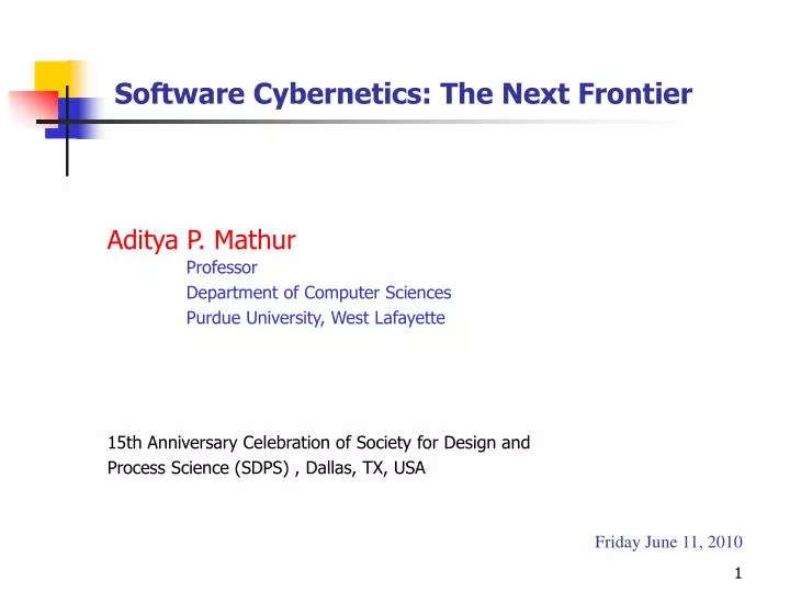
Software Cybernetics: The Next Frontier. Aditya P. Mathur Professor Department of Computer Sciences Purdue University, West Lafayette. 15th Anniversary Celebration of Society for Design and Process Science (SDPS) , Dallas, TX, USA. Friday June 11, 2010. Collaborators.

E N D
Software Cybernetics: The Next Frontier Aditya P. Mathur Professor Department of Computer Sciences Purdue University, West Lafayette 15th Anniversary Celebration of Society for Design and Process Science (SDPS) , Dallas, TX, USA Friday June 11, 2010
Collaborators Kai-Yuan Cai, Beijing University of Aeronautics and Astronautics Joao Cangussu, Microsoft Ray DeCarlo, Purdue Scott Miller, Purdue
Key Question Can we model and control a software development process using theories and techniques available to control engineers?
What is Software Cybernetics? A (new) discipline that aims at the development of models and control methodologies for software and the software development processes.
Focus of Software Cybernetics • Formalization and quantification of feedback mechanisms in software processes and systems • Adaptation of principles and techniques of control theory to software processes and systems • Application of the principles of software related theories and engineering to control systems and processes • Integration of the theories of software engineering and control engineering
Software and Control • Software • Code • Development • Maintenance • Evolution • Control • A finite or infinite sequence of actions applied to the controlled object to achieve a given apriori goal for the controlled object.
Software Cybernetics: Domain Modeling and Simulation: Abdel-Hamid and S.E. Madnick. Software Project Dynamics. Prentice Hall 1991. Role of feedback in software evolution [Basili et al. 1994; Lehman, 1996]
Software Cybernetics: Domain Modeling and control for decision support: Software synthesis [Sridharan et al. 2003] Software test process control [Cangussu et al. 2002] Adaptive testing [Cai 2002] Software development process control, incremental lifecycle model [Miller et al. 2008]
Software Cybernetics: Domain Modeling and control for reliable operation: Eliminating Concurrency Bugs with Control Engineering [Kelly et al. IEEE Computer 2009]
Required Quality + Effort - Observed Quality f(e) Additional effort What is f ? Feedback Control: The basic idea Specifications Program
Software Development Process: Definitions A Software Development Process (SDP) is a sequence of well defined activities used in the production of software. An SDP usually consists of several sub-processes that may or may not operate in a sequence. The Design Process, the Software Test Process, and the Configuration Management Process are examples of sub-processes of the SDP.
Requirements Analysis Design Code/Unit test Integrate/Test System test More test Deploy Software Development Process: A Life Cycle Techniques proposed here can be adapted to any life cycle model. Requirements Elicitation Not all feedback loops are shown.
Study 1: Modeling the system test phase Software Test Process (STP): System test phase; physical system analogy Objective: Control the STP so that the quality of the tested software is as desired. • Quantification of quality of software: • Number of remaining errors • Reliability
Study 2: Modeling the development process Software Development Process (SDP): All phases, queuing system anaogy [Miller et al. COMPSAC 2004] • Objective: • Offer change suggestions capable of achieving a specified deviation from the predicted system trajectory. • Quantification of quality of software: • Number of remaining errors • Reliability
The System Test Phase: Parametric Control Cangussu et al. TSE 2002
r0 observed Approximation of how r is likely to change r - number of remaining errors schedule set by the manager rf t- time cp2 cp3 cp4 cp5 cp6 cp7 cp8 cp9 cp1 t0 deadline Problem Scenario cpi = check point i
sc r0 robserved(t) wf+wf Actual STP + ’ wf w’f wf+wf STP State Model + sc r0 Our Approach + Initial Settings (wf,) rerror(t) Controller Test Manager + rexpected(t) wf: workforce : quality of the test process
Software Block Xcurrent Spring Force Effective Test Effort X: Position Mass of the block Viscosity Quality of the test process Number of remaining errors Software complexity Physical and Software Systems: An Analogy Dashpot External force To err is Human Rigid surface Spring Xequilibrium
Physical Systems: Laws of Motion [1] First Law: Every object in a state of uniform motion tends to remain in that state of motion unless an external force is applied to it. Does not (seem to) apply to testing because the number of errors does not change when no external effort is applied to the application.
.. r CDM First Postulate: The relationship between the complexity Sc of an application, its rate of reduction in the number of remaining errors, and the applied effort E is E=Sc. Physical Systems: Laws of Motion [2] Newton’s Second Law: The relationship between an object's mass m, its acceleration a, and the applied force F is F = ma.
Physical Systems: Laws of Motion [3] Third Law: For every action force, there is an equal and opposite reaction force. When an effort is applied to test software, it leads to (mental) fatigue on the tester. Unable to quantify this relationship.
CDM First Postulate The magnitude of the rate of decrease of the remaining errors is directly proportional to the net applied effort and inversely proportional to the complexity of the program under test. This is analogous to Newton’s Second Law of motion.
CDM Second Postulate Analogy with the spring: The magnitude of the effective test effort is proportional to the product of the applied work force and the number of remaining errors. Note: While keeping the effective test effort constant, a reduction in r requires an increase in workforce. for an appropriate .
CDM Third Postulate Analogy with the dashpot: The error reduction resistance is proportional to the error reduction velocity and inversely proportional to the overall quality of the test phase. for an appropriate . Note: For a given quality of the test phase, a larger error reduction velocity leads to larger resistance.
Force (effort) balance equation: . x(t) = Ax(t) + B u(t) : Disturbance State Model
Given: r(T): the number of remaining errors at time T r(T+T): the desired number of remaining errors at time T+T Question: What changes to the process parameters will achieve the desired r(T+T) ? Computing the feedback-Question
Obtain the desired eigenvalue. Computing the feedback-Answer From basic matrix theory: The largest eigenvalue of a linear system dominates the rate of convergence. Hence we need to adjust the largest eigenvalue of the system so that the response converges to the desired value within the remaining weeks (T). This can be achieved by maintaining:
Given the constraint: Computing the feedback-Calculations (max) Compute the desired max We know that the eigenvalues of our model are the roots of its characteristic polynomial of the A matrix.
We use the above equation to calculate the space of changes to w and such that the system maintains its desired eigenvalue. f Computing the feedback-Calculations (max)
Computing the feedback-Input to the Manager The space of changes in the workforce and the quality of the process is made available to the test manager in the form of suggestions for possible process changes. The test manager may decide to select a combination of these values for implementation or simply ignore them. In each of the two commercial studies we carried out, the manager ignored the suggestions given using the model.
Case Study: The Razorfish Project Project Goal: translate 4 million lines of Cobol code to SAP/R3 A tool has been developed to achieve the goal of this project. Goal of the test process: (a) Test the generated code, not the tool. (b) Reduce the number of errors by about 85%.
continue testing yes = output 2 output 1 no run run modify SCobol Transformer SSAP R/3 input Select a Test Profile Razorfish Project Test Process
Expected behavior Project data Prediction using the model Prediction using feedback 85% reduction achieved. Razorfish Project: Results (intermediate) If the process parameters are not altered then the goal is reached in about 35 weeks.
Alternatives from Feedback: STP Quality Improving quality alone will not help in achieving the goal. Desired eigenvalue=-0.152
Desired eigenvalue=-0.152 Alternatives from Feedback: Workforce Changing the workforce alone can produce the desired results.
Alternatives from Feedback: STP quality and workforce Set of valid choices for changing the quality and the workforce
Razorfish Project Results (final) The project was completed in 32 weeks. The model predicted 85% error reduction in 35 weeks.
The incremental development process: Queuing model and control Miller et al. COMPSAC 2008
Interconnected dynamical systems* C1 C2 C4 u y C3 C: Component (sub-system) u: System input y: System output x: System state vector *DeCarlo and Saeks, 1980
Incremental software development: Components R R: Requirements
System of systems model L11: Linear feedback from sub-system system outputs to sub-system inputs L12: Entry of external inputs into subsystem inputs L21, L22: Similar relationships for system outputs
Workforce productive capability : productivity measure : workforce size : remaining work items : process quality : calibrated average productive capability/FTE
Productivity state model: behavior Cangussu et al. [2002] (Csikszementmihalyi, 1988)
State model of a queue a1 a2 (x1) b1 b2 (x2) b3 (x3)
Coordination constraints x: features coded c(x): step function; test case execution threshold Cubic splines used for smoothing the threshold function.
Additional models Defect introduction: Based on Barry Boehm’s COQUALMO model Defect detection; failure analysis: Lotka-Volterra predator-prey population dynamics model Proportional splitting model: defects in code versus defects in test case code
Simulation study: System description • Incremental development process • Two serial increments • First increment: • 10 features, 70 tests, 70 regression tests • Second increment: • 20 features, 130 tests, 130 regression tests • 29 FTE: • 5 assigned to each development activity except feature and test correction that are assigned 5 each.