Calibration Tutorial: Discovery32

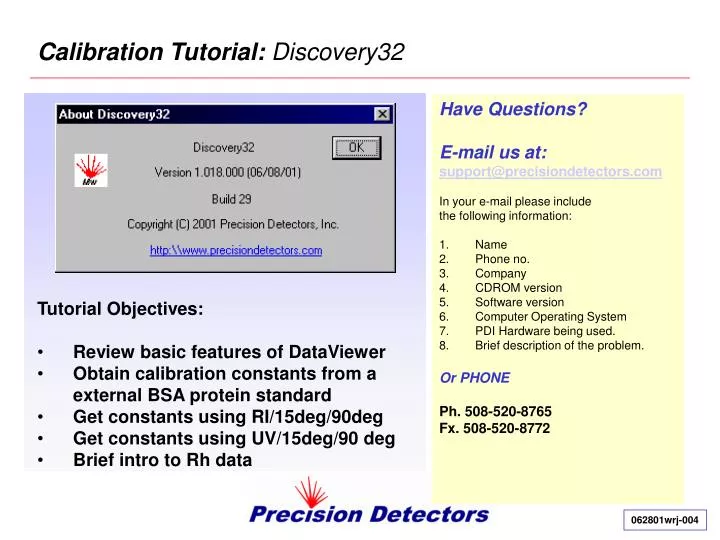
1. Calibration Tutorial: Discovery32 • Have Questions? • E-mail us at: • support@precisiondetectors.com • In your e-mail please include • the following information: • Name • Phone no. • Company • CDROM version • Software version • Computer Operating System • PDI Hardware being used. • Brief description of the problem. • Or PHONE • Ph. 508-520-8765 • Fx. 508-520-8772 • Tutorial Objectives: • Review basic features of DataViewer • Obtain calibration constants from a external BSA protein standard • Get constants using RI/15deg/90deg • Get constants using UV/15deg/90 deg • Brief intro to Rh data 062801wrj-004

2. Experimental Conditions Standard: BSA (2 mg/mL) cat# Sigma P-0834 Column: YMC-Pack Diol-300, 300 x8 mm ID, 5 um silica cat.# DL30S05-3008WT Eluent: Phosphate buffered saline 120 mM NaCl, 2.7 mM KCl, 10 mM phosphate buffer Sigma Diagnostics #1000-3 Flow rate: 1 mL/min Injection vol.: 100 uL Order of detection:FIRST UV @ 280 nmSECOND LS (15 deg, 90 deg, Rh) THIRD RI The light scattering detectors were built inside a Waters 410 RI ( PD 2020DLS inside) The UV was a Waters 484 Tunable Absorbance Detector which was plumbed to the Waters 410 with the shortest 0.007” ID peek tubing . A PDI low dispersion inline filter was placed between the column and the first detector. The inline Filter was fitted with a 13 mm diam., 0.2 um Supor membrane. Data acquisition: The UV channel was assigned to the the spare input channel. Acquisition Rate was 1 Hz (sample interval 1 second), with a collection fraction of 0.1.

3. Backgrounder This tutorial is intended to be a quick “graphically oriented” approach to obtain calibration constants for your HPLC/Light scattering (LS) detection system. The separation mode is typically based on size exclusion and is typically called size exclusion chromatography (SEC) for aqueous based columns and solvents and gel permeation chromatography (GPC) for non-aqueous based solvents and columns. The following slide lists the key attributes of the calibrant and the chromatographic system that contribute to reliable calibration constants. These detector constants are required, along with knowing the response factors for the concentration of the standard for determining accurate molecular weights and their distributions when using laser light scattering detection. Although there are several approaches that have been implemented for calibration of laser light scattering detectors, the PDI detection system uses the external standard approach as it is straight forward and can be done with eluents that are compatible (if not identical to your actual running method). Even if you selected a standardization mode that was chemically dissimilar to your actual running method. [ e.g. calibration was performed using a polystyrene standard on a GPC column running tetrahydrofuran (THF) and the actual running method was running a SEC column with a phosphate buffered saline (PBS) eluent ] the calibration constants would virtually be the same (provided the conditions on the following page were observed). This tutorial will first provide an overview of the new Discovery32 user interface which is dramatically different to the former PDI data analysis program “PrecisionAnalyze”. Calibration for RI and LS is performed first with a bovine serum album (BSA) chromatogram, followed by UV and LS. The approach is to select your calibration mode, establish baselines for each of the traces, integrate the standard peak and determine the calibration constants.

4. What constitutes a good standard? The Standard 1. The material is of known Mw 2. Known concentration 3. Monodispersed (Mw/Mn 1.00 to 1.01) 4. An isotropic scatterer*. 5. Should preferably be free of aggregations 6. The dn/dc of the standard is required (if not known, it can be determined using the RI detector) 7. The extinction coefficient of the material at the monitoring wavelength is required when using UV as the concentration source. The Chromatography 1. Standard should chromatograph as a single peak. 2. Recovery of standard should be 100% 3. Enough material must be injected to obtain good signals from both LS and concentration source detectors. 4. If aggregates exist, the standard peak must be resolved from the aggregations. 5. The standard peak must also be resolved from terminal peak (small Mw impurities). The Eluent 1.The refractive index of the eluent at the temperature of the detector cell is required when using 15 degree LS in the Mw calculations. 2. The viscosity in (poise) of the eluent at the temperature of the detector cell is required for Rh determinations. *The Mw should be large enough to generate a sufficient light scattering signal but not so large that the 15 and 90 degree signals are not of equal intensity. For globular proteins non-isotropic scattering begins as the material approaches 1 million daltons. Typical protein standard for aqueous SEC: bovine serum albumin (66.5 kD) Typical room temp GPC standard for THF solvents: polystyrene (96.4 kD polydispersity 1.01)

5. Procedures for Calibration (Get raw data for standard) UV trace for peak standard (first detection series) 15 and 90 degree peak for the standard (simultaneously obtained and second in series) RI trace of standard peak (last in series because of cell backpressure limitations) Response These peaks are offset by the amount of inter-detector volume between the cells. The time differential is dependent on the flow rate of the eluent, the volume remain constant as long as the tubing connections between detectors is not changed. Time (Elution volume)

6. Outline of Procedures for Calibration (Establish baselines) UV trace 15 degree static trace 90 degree static trace RI trace Response Establish baselines for each of the peaks Baseline for UV Baseline for 90 degree static Baseline for 15 degree static Baseline for RI Time (Elution volume)

7. Outline of Procedures for Calibration (Get Interdetector volumes) Offset zero (reference: LS detectors) Neg. offset for UV Pos. offset for RI After baselines the inter-detector volume (IDV) is automatically determined by the “det. Cal constants” routine. The algorithm requires baselines and integration region encompassing the one concentration source detector and one or more of the LS detectors. UV/LS and RI/LS are determined separately as they have different integration regions. Response Integration Region for UV and LS Integration Region for RI and LS Time (Elution volume)

8. Outline of Procedures for Calibration (Apply newly determined IDV’s) Offset zero (reference: LS detectors) When the IDV have been properly determined the concentration source detectors line up with the light scattering detectors. Response Time (Elution volume)

9. Outline of Procedures for Calibration (Regionally height normalize) To better visualize the alignment , the traces can be regionally height normalized . Response Time (Elution volume)

10. Launch the program after installing onto computer Double Click the Discovery Icon to launch program Or from the short cut found in Start/Programs/PrecisionDetectors/Discovery32

11. DataViewer: Selecting a Directory Discovery32 opens up into a DataViewer window. This window allows you to ascertain running conditions for the chromatogram and to get a preview of the files without having to open each one up for examination. You may select the directory to preview by clicking the “Change>>>” button. A dialog box will appear where you may select the directory of choice. The path of the directory will be shown in the box to the right of the “Change>>>” button. You must use the “Change>>” button to select a directory instead of typing in the path box.

12. DataViewer: Previewing a File This line was highlighted simply by clicking once on the name. The chromatogram with all of the collected channels of data are shown in the small preview window (upper right hand corner).

13. DataViewer: Sorting Files Date and time the file was collected. Info description “sample”, “eluant”, “info” etc are found starting here and scrolling right.. RLHSC represents the channels collected R = Rh (not RI) L = (low) = 15 degree H = (high) = 90 degree S = (spare) = UV C = (concentration) = RI Files may be sorted by filename, eluant, sample name, dn/dc or by date. The run conditions for each file are found in a scrollable row.

14. DataViewer: Tool Bar and Status Bar TOOL BAR The Tool bar and Status bar may be enabled or disabled for viewing. STATUS BAR

15. DataViewer: Changing Location and Shape of Toolbar TOOL BAR can be dragged from it’s standard position and can float as a separate window which can be reshaped to meet your preferences. The TOOL BAR can be covered or hidden with other Discovery32 windows, make sure you place it in a convenient corner for best access.

16. DataViewer: Loading a Chromatogram The other way is to go to File..Open or Click the “Open Folder Icon Button” One way to load a chromatogram is to double click on the file in this box. The file loaded will be acknowledged by having the line selected turn red AND where the red ovals have been placed.

17. DataViewer: Loading a Chromatogram (Continued) Remember: If you single click another file, that line will be highlighted with dark blue and an UNLOADED chromatogram will be seen in the preview window above (right). The actual loaded file will be identified by the red highlighted text and the places where the ovals are shown.

18. DataViewer: Viewing the Loaded Chromatogram A processing window for the loaded chromatogram can be accessed by clicking this button. This is the “chromatograms” window. The sample name is the only information the default conditions will display unless the report selection fields have been properly checked. See next slide.

19. Report Selection: Placing File Name on Chromatogram It is recommended that the following items be selected in the Report Selection Menu. It will show the file name on the chromatogram window. If the “Add File Name to Footer” is not checked, you can only determine what file you are looking at by the file name in the DataViewer footer or in Summary section of the Results window.

20. Report Selection: File name The file name shown here will not match the file name loaded if the file that was loaded was “saved as” with a different name. The original name is shown here. The “saved as” file name is shown in the “status bar”

21. Helpful Hint 1: Optimizing Window Size The “chromatograms” window is the only resizable window. Making the window larger makes it easier to perform functions such as baseline and integrations. Place the Tool bar over here and in full vertical view. Then grab a corner of the chromatogram window and drag it to a larger size. (Leave enough room to see the tool bar). (Note: Leave window open, if you close it and decide to reopen it again, it will default back to the original size)

22. Optional: Changing Display Settings If you prefer to have a chromatogram window with a white background follow the procedure below.. On the computer desktop go to Start/Settings/Contol Panel/Display The window (Display Properties) go to the Appearance tab select “HIGH CONTRAST WHITE”. Hint: A quick way to get to this screen is to right mouse click the Windows desktop.

23. Optional: Changing Display Settings (high contrast white) This is an example of what “high contrast white” looks like.

24. The Tool Bar Open Overlay Display Window These three buttons will be addressed in a future tutorial Open Branching and Structure Window Open Conventional GPC Window Open Results Window These are the three buttons we will need to use for calibration Open Calculation Set Window Open Chromatogram Window Start Acquisition Software Print If more than one copy or version of Acquire32 is found, a dialog box will pop up asking for your selection Save Open

25. Chromatogram Window Each of the pop-up windows has click on tabs where you can get to different features. For the purposes of this tutorial we will use only the “Operate On Chromatograms” TAB

26. Set Up Calculations Window (Options) SETTING UP TO CALIBRATE Detector Calculations: RI/ Light Scattering Mw Smoothing: None Calculation Types: Mw Calculations (15 & 90 degree) PD2020 Rh Calculations: Yes Laser Wavelength: 809 nm (If you have Rh capability your laser is 809 nm, if you do not have Rh capability you need to refer to your Calcert document for the actual wavelength of the laser used in your instrument). If you are uncertain or believe your unit was upgraded, contact PDI and provide them

27. Set Up Calculations Window (Detectors) SELECTING THE DETECTORS TO DISPLAY By clicking on the “Detectors” tab of the Setup calculation window, you can select the detectors to display. To simplify the viewing we will not visualize UV and Rh data when performing baselines and integrations on the chromatogram found in the “Chromatograms” window. NOTE 1: The tabs are placed in order of how you would set up your calculations. Options, Detectors, Constants and finally Determine Cal Constants. NOTE 2: If you select a channel and check both left and right y-axis, the left axis is displayed only. If you select a left y-axis for 90 and a right y-axis for RI, there will be two y axes shown.

28. Set Up Calculations Window (Constants) 1 of 2 The Run RI and Run UV constants shown on the left side are the current constants being applied to the chromatogram. These constants are stored with the file that is opened. The right side constants are the instrument values. These constants are not stored with the file but are stored in Discovery32. Every time a new file is opened with this program, the same instrument constants will also appear. When you calibrate a file or update constants through the Determine Cal Constants routine, both left and right side columns are updated. If you wish the new constants to be associated with data files to be collected. These constants can be copied and pasted in the Calibration fields found in PrecisionAcquire32. Calibration constants can be manually entered into the fields if you have the information available. The right arrow (RI)buttons when clicked copy the contents of the Run RI side to the Instrument RI side. The left arrow (RI) buttons transfer the constants from the Instrument RI side to the Run RI side. The Run UV arrow buttons perform similar functions. The “update” button activates every time a manual change occurs. When you click “update” ,a dialog box will pop up asking if you wish to save settings or cancel..

29. Set Up Calculations Window (Constants) 2 of 2 IMPORTANT: The Cal solvent index is the RI constant of the solvent that was used during a calibration. It does NOT update when the solvent index is changed in the Results summary page. It will only update if a new calibration has taken place and will obtain the new value from the eluent RI field of the “Determine cal constants” field. If you are doing Mw calculations using two angles and the solvent has changed for the method, you must enter the NEW solvent index here also. If you recently updated the cal constants for a file that is currently opened (run side column) and you wish to have these same values applied to another set of files with older constants. Simply click this button and select up to 20 files (at a time) by holding the ctrl button down and clicking the file names you wish to modify. A dialog box will confirm how many files were modified. Alternatively, if you modified constants through the “determine cal constants routine” the new constants will also be found in the instrument side column. You can then transfer the instrument constants to the run constants side by clicking the left pointed arrows.

30. Setup Calculation Window (Determine Cal Constants) Upon viewing this screen, all the constants are blank here. This occurs if you have not established baselines and integration regions for the chromatograms. Lets establish baselines and integration regions so that we can obtain new constants.

31. Chromatogram Window: Establishing Baselines (1 of 3) Right mouse click (once or twice) until a pop-up selection box appears. Select Set baseline. This dialog box then appears. Deselect Spare Detector then press OK. Continue onto next slide NOTE: Low Angle Scatter = 15 degree Channel High Angle Scatter = 90 degree Channel Spare Detector = (Typically reserved for UV)

32. Chromatogram Window: Establishing Baselines (2 of 3) start end The pointer converts to a cross-hair icon. Starting with a flat portion on 90 degree and RI before the peaks, click and hold the left mouse button down and drag it to a similarly flat region to the right of the peaks. Release the mouse. If you, like what you have selected, move your cursor to a region between the two vertical black lines (start and stop of baseline determination) and right mouse click. If you do not like the selection, right mouse click outside that region.

33. Chromatogram Window: Establishing Baselines (3 of 3) If you want to move a baseline marker. Hold the CTRL button down then left mouse click and hold the marker you wish to move. Drag the marker to where you wish to move it to and release. Baseline markers shown

34. Chromatogram Window: Normalizing Region Before selecting integration regions for calibration, it is better to normalize the heights of the various traces of the standard peak. Right mouse click (once or twice) until a pop-up selection box appears. Select Normalize Region. Select the region you want to normalize (exclude negative peaks). Similar to what you did with baseline selection. Right mouse click inside the vertical black lines to select.

35. Chromatogram Window: Zooming on Normalized Region Take your cursor (pointer) . Hold the left mouse button down and drag diagonally across the region you wish to zoom into. Then release mouse start end

36. Selecting Integration Region Right mouse click (once or twice) until a pop-up selection box appears. Select Set Integration Region. Hold and drag the cross hair cursor (left mouse button) over the monomer peak region of BSA and release. ( You may have to re-zoom in after this operation) Integration marks shown

37. Determine Cal Constants: (1 of 5) In the previous chromatogram, baselines and integration of the main peak have been performed. We can now proceed with obtaining calibration constants. FIRST:Check that all of the fill-in fields information are correct. The Mol. Wt. entered in as the full number (e.g 66500 not 66.5 kD). Make corrections where necessary. SECOND:The quality factor should be 0.98 to 1.00 before accepting the inter-detector volume. (Make sure you have measured the flow rate to confirm that what is programmed into the pump is actually what the pump is delivering.) If the value is lower than 0.98, try reintegrating a wider or narrower integration region. If it still did not improve, rerun the standard and or check to make sure it is monodispersed (pure). . THIRD: If the quality factor is adequate then click ALL then click Apply. If the standard consisted of a solitary peak the calibration is essentially completed. Since our BSA standard does have measurable dimer, trimer and higher order aggregates we have to expand our integration region to include the total area of these peaks so that an accurate concentration constant (RI or UV) is obtained . After which the monomer region is reintegrated to optimize 15 and 90 constants.

38. Determine Cal Constants/ RI Constant (3 of 5) FIFTH:Expand the integration region to include all of the RI area (terminal peak at 12 minutes excluded). The 2 mg/mL is distributed over RI aggregates and monomer.

39. Determine Cal Constants/ RI Constant (4 of 5) SIXTH:Go back to Det. Cal Constants after reintegrating the RI peaks. Click Accept then click Apply NOTE: PrecisionAnalyze will report RI constants ranging from 75000 to 85000 and are not compatible with Discovery32 which typically has a RI constant around 3. .

40. Determine Cal Constants/ 15 & 90 degree constant (5 of 5) SEVENTH: Reestablish integration for monomer, then proceed to complete the 90 degree constant. Select the start region somewhat away from the trough between the dimer and monomer peak as the dimer is tailing a little into the monomer. Then accept the 15 and 90 degree constant. Then click apply. We have now calibrated the RI, 15 and 90 channels.

41. Checking your results (1 of 2): Run Params Calibration of the monomer BSA peak is correct for RI/15 and RI/90 The entered dn/dc is 0.1670 the software suggests that this value should be 0.1451 if the area of the monomer peak was precisely 2 mg/mL. This is not the case as the 2 mg/mL is distributed over the several peaks. The entered concentration is 2 mg/mL, the calculated concentration for the monomer peak is 1.7381 mg/mL which is correct as that is the portion of monomer distributed between aggregates. By checking this box, Batch calculations will then read 66.5 K

42. Checking your results (2 of 2):Summary Avg. Mw for BSA for the integrated slice. The heart-cut of the monomer peak is very monodispersed at 1.001 The peak (apex) molecular weight is shown here

43. Field Information Update NOTE: An extra line of information has been included n the Run Information window. The original file name (source file) and its new name (If it has been modified and saved as) is now displayed together..

44. Checking the BSA Dimer peak for Mw Integrate the center region for dimer of BSA and check Mw. The calculated molecular weight for this peak is 2.02 x that of the calculated Mw for monomer.

45. Checking the BSA Trimer peak for Mw Integrate the center region for trimer of BSA and check Mw. The calculated molecular weight for this peak is 2.98 x that of the calculated Mw for monomer.

46. Checking the BSA Tetramer peak for Mw Integrate the center region for tetramer of BSA and check Mw. The calculated molecular weight for this peak is 4.17 x that of the calculated Mw for monomer.

47. Determining Large Aggregation BSA Integrate the full RI area region. The avg. Mw is 74.5kD with a polydispersity of 1.057

48. Looking at the Mw vs Elution Profile The Mw vs Elution Profile helps to visualize the Mw variations across a peak. Here both monomer and dimer show very good consistancy as indicated also by the polydispersity factor.

49. Calibrating the UV Detector and LS Channels (1 of 6) Now that we have successfully calibrated the BSA chromatogram using RI/Lightscattering, lets proceed to complete the calibration using the UV/Lightscattering option. Select “UV/Lightscattering Calculations” Disable viewing the RI channel and enable the UV channel. Check both left and right y-axis buttons for the UV

50. Calibrating the UV Detector and LS Channels (2 of 6) We only now need to establish baseline on the UV trace since the other channels have been already operated on. Select only the “spare detector” which is the UV channel. Then click OK. Select and drag the cross hair cursor on a flat region before the first lift off of UV baseline and well after the landing on the UV trace. (3 minutes to 14 minutes.)