Download
1 / 56
560 likes | 702 Views
Physical Modelling of Concentration Fluctuation s in Simple Obstacle Arrays. Robert Macdonald and Brian Kim Department of Mechanical Engineering University of Waterloo, Ontario, Canada Eric Savory Department of Mechanical and Materials Engineering University of Western Ontario, Canada

E N D
Physical Modelling of Concentration Fluctuations in Simple Obstacle Arrays Robert Macdonald and Brian Kim Department of Mechanical Engineering University of Waterloo, Ontario, Canada Eric Savory Department of Mechanical and Materials Engineering University of Western Ontario, Canada Miho Horie and Shiki Okamoto Shibaura Institute of Technology, Tokyo, Japan Presented at NATO ASI, May 2004
Content • Background • Description of the physical modelling facility - Hydraulic flume - Atmospheric boundary layer simulation - Obstacle arrays • Planar Laser Induced Fluorescence (PLIF) technique for concentration measurements • Discussion of results for - Mean concentrations - RMS concentration fluctuations • Conclusions
Air Pollutants • Local stack plumes • Exhausts from automobiles • Accidental Releases
Street Canyon • Geometry created bya narrow street with • buildings lined upcontinuously along both • sides (Nicholson, 1975) • The canyon flow is affected bythe arrangement • and spacing between the buildings
Background Concentration fluctuations can be important in assessing toxic risk. Experimental data on concentration fluctuations in obstacle arrays is quite sparse. It has been suggested that Crms is O(Cmean) but estimates vary greatly. The present study seeks to quantify Crms / Cmean for different obstacle arrays and downwind locations.
Objectives • Obtain concentration profiles using PLIF technique in a water flume • Determine the effects of obstacle configuration on mean dispersion parameters (max. concentration, plume height, etc.) • Obtain relative concentration fluctuation intensity profiles • Validation of PLIF application
Scale Modeling • Full-scale (field) and Small-scale Studies • 10 m : 5 cm = 200 : 1
Hydraulic Flume Fully developed, turbulent approach flow (10cm/sec) Experimental Facilities (I) 2.4 m - Flume dimensions: 12.6 m x 1.2 m x 0.8 m
Light Source System Argon ion Laser (Maximum, 5W) Fixed frequency resonant optical scanner 1 mm Light sheet Experimental Facilities (II)
Approach Flow Characterization • Acoustic Doppler Velocimeter (ADV: 20 Hz) Reference Height (5cm) Zo = 0.20 mm (0.4 m FS) UH = 5.74 m/s U* / UH = 0.13 = 0.29 Suburban terrain
Non-dimensional Turbulence Intensity X = 50 cm X = 0 cm
Longitudinal > Lateral > Verticalturbulence Intensity X = 147 cm X = 100 cm
Dispersion Parameter (I) • Non-Dimensional Concentration (Kc) • Can be directly • compared with • non-dimensional data • from • field-scale experiments • or • dispersion data from • other wind tunnel • facilities Where CN = C/Cs Q = Volume flow rate UH = Velocity at H (5cm) Cs = Source conc.
DispersionParameter (II) Reference : Lecture Not (Air Pollution) Z/H • Net vertical plume variance Vertical rise of the plume is a combination of two factors; The centre of the distribution Zc and the standard deviation of the distribution sZ z/H C (z)
Experimental Configuration (I) • Square and Staggered Building Array
Experimental Configuration (II) • Unobstructed plume - Less dilution than in the obstacle arrays higher concentrations - A baseline case for comparison to the obstacle (building) array results “Lego” roughness Nuts
Experimental Configuration (III) • 2-Dimensional with different Area Density AF = Frontal area AT = Total plan area 0.5 H 1.5 H H2 / (2.5Hx2.5H) = 16% H2 / (1.5Hx1.5H) = 44%
Previous work with these arrays • ADV measurements of mean velocity and turbulence quantities, Carter (2000), Macdonald et al (2002). • Correlation of turbulence quantities above obstacles with: u / U* = 2.10, v / U* = 1.65 and w / U* = 1.20. • Peak TKE about 30% greater above staggered array when compared to square array. • Value of about 50% larger for flat plate arrays compared to cube arrays.
Source Release System • 3 different heights (0.3 H / 0.5 H / 1.0 H)
Source Types and Downstream-Scale Upstream source (spacings from f = 16%) 1 row 2 row 4 row 6 row U 2.25H 4.75H 9.75H 14.75H Inside source U
Summary of Experiments Source Types Upstream Inside Array Types Square 16 % 44 % 16 % (Source Height 0.3H,0.5H,1.0H) Staggered 16 % 16 % Two Dimensional 16 % 33 % 44 % 16 % Unobstructed With NUTS and LEGO
Traditional Point Measurement Techniques • Allow measurement of • Transport processes • Spatial distribution • of concentration and • velocity
57 77 71 65 67 55 76 76 70 65 65 53 78 78 70 63 63 61 75 75 77 68 58 57 38 33 27 27 58 38 30 33 23 15 57 47 41 35 25 5 56 46 40 35 25 13 58 48 40 33 23 11 55 45 37 28 18 17 95 95 83 99 99 93 81 97 98 98 87 Optical Measurement using Planar Laser Induced Fluorescence (PLIF) • DigitalCCD camera - Whole field measurement • Indirectmeasurement - Using dye (as tracer) • Non-intrusive - Optical technique
The basic PLIF system Planar laser light source Fluorescent tracer release system Digital image acquisition and storage system Digital image analysis software PLIF Components 1 2 3 4
PLIF Principle • The higher the concentration (C)of dye, the greater the intensity of emitted light (E)for a given intensity ofincident light (I): • = calibration const. • (e.g. Crimaldi & Koseff, 2001) • Allows measurement of the spatial distribution of tracer concentrations Inside test section of water flume
In the experiments, only the fluorescent colour (555 nm) of dye is visible to the CCD camera the use of a filter removes background argon-ion laser light (514nm) Low-Pass Filter
Calibration • PLIFtechnique requires a careful calibration to • convert image intensity to concentration. 0.5 0.25 0.1 0.05 (ppm) KNOWN Concentration • To obtain the actual concentration, a calibration • box was used with known concentrations of dye • to form a calibration curve
Set-Up Experiment Configuration Image Grabbing Image Recording In each ROI Calculating Concentration With Calibration Calibration Box Image Record Collecting Concentration Profile Data Data Analysis Procedure Experimental Work Image processing Data Analysis Mean Concentration Using Gaussian C.Fit Extract Dispersion Parameter Analysis Of Relative Concentration
Image Gathering • Instantaneous Images : 1st ~ 20th ( 15 sec interval ) Average Image
Mean Concentration ( C ) Turbulent ImageManipulation • Fluctuating concentrations: Fluctuating Concentration ( C ) Instantaneous Concentration ( C ) - = - = Turbulence Image Instantaneous Image Average Image
Fluctuating concentration Image • Turbulence Variance • (s2 ) • Turbulence RMS (s )
Concentration Data Analysis Variance (s2 ) 6.5 6.5 10.9 15.1 11.1 15.1 5.3 5.3 9.3 8.4 9.4 14.7 5.9 5.9 9.4 15.1 11.1 11.1 1.4 1.4 7.4 10.9 10.9 11.7 4.4 4.4 9.3 9.1 9.1 11.1 5.8 5.8 8.4 9.4 9.4 11.7 78 78 83 87 87 88 78 78 80 83 83 85 77 77 81 85 85 85 76 76 80 85 85 83 78 78 80 83 83 81 75 75 77 78 78 77 Concentration Image Intensity RMS (s ) Mean (C)
Number of Images for Analysis • No significant influence of image sample size on the Average image for Cmean Z/H = 1 Present Study
Appropriate sampling time = 5 minutes to ensure • reliable data for Concentration fluctuations Crms Z/H = 1
Results • Mean Concentration Profiles • Non-Dimensional Concentration • Analysis of characteristics for the various area densities and configurations • Concentration fluctuation profiles
Averaging Partitioning • Mean concentration profiles - Each canyon was divided into 5 sections Mean Concentration Image
20 pixels 0.0077(at Z/H=0.7) Average • Spatial Averaged Concentration - Upstream Staggered 1st Canyon Example 20 pixels 100 pixels
4 1 2 3 4 6 G 1 2 G 2 G 4 G 6 1 0 0 0.1 0.2 0.3 0.15 0.25 0.05 • Mean concentration profile fitted with Gaussian curve Z / H (ppm) C(z)
Summary of considerations • Saturation, Attenuation, Non-linear regression , Distortion, Reflection, Images for analyzing • Control Factors • Source concentration (24.5 ppm) • Small aperture (narrow field of view) • Weak dye ( C <= max ~ 0.5 ppm) • Gaussian curve fitting parameters • Maximum length of camera position (3.8 m) • Painting all blocks black • 5 minute sampling with 20 images is optimal 0.5 ppm
I. Comparison of dispersion parameters (Kc, Zbar) with Wind tunnel and Point measurement data • Different configuration for two experiments • 1. Wind T : Ground level release • Point measurement at centre • of canyon • 2. Flume : 0.5 H release,at centre of canyon
Upstream Square Array f = 16% Point Measurement Wind Tunnel Measurement
Upstream Square Array f = 16% Point Measurement Wind Tunnel Measurement
II. Analysis of dispersion parametersKc, Zbar With MEAN CONCENTRATION
Upstream Source (lf = 16%) Initial plume disperses most rapidly for 2D array and least for square array. Similar trends for inside source.
Upstream Source (lf = 16%) Resulting concentrations lower for 2D canyon compared to others.
III. Analysis of fluctuating concentrations With Relative CONCENTRATION (Crms/Cmean)
Upstream Square 16 % Relative Concentration Profiles • The peak of the relative concentration fluctuation intensity (Crms/Cmean) occurs in the mixing layer immediately above the obstacles • The ratio (Crms/Cmean) decreases rapidly below rooftop height.