Download
1 / 70
700 likes | 714 Views
Optimal and Information Theoretic Syntactic Pattern Recognition. B. John Oommen Chancellor’s Professor Fellow: IEEE ; Fellow: IAPR Carleton University, Ottawa, Canada. Joint research with R. L. Kashyap. Y. Traditional Syntactic Pattern Recognition. Noisy Pattern: To be Recognized

E N D
Optimal and Information Theoretic Syntactic Pattern Recognition B. John Oommen Chancellor’s Professor Fellow: IEEE ; Fellow: IAPR Carleton University, Ottawa, Canada Joint research with R. L. Kashyap
Y Traditional Syntactic Pattern Recognition Noisy Pattern: To be Recognized Compare Y with the set of Patterns. Using Traditional Edit Operations: • Substitutions. • Deletions. • Insertions.
F I G H T F I G H T F I G H T S S S N N N I I I P P P String-to-String based – DP Matrix
String-to-String based – DP Dynamic Programming (Age-Old) : D(Xi , Yj) = Min[D(Xi-1 , Yj-1) + d(xi yj) , D(Xi , Yj-1) + d( yj) , D(Xi-1 , Yj) + d(xi)]
F I G H T S N I P String-to-String based – Calculation
X Y = = f n i i g g h h t t s Example • Consider: • Question: How far is X → Y? D(X,Y)
Example • Measured Symbolically by How much “work” is done in editing X → Y • Substitutions. • Deletions. • Insertions. Best score: D(X,Y)= d (f → n) +d (s →λ). Depends on the individuals distances. • d (f → n). 3.1 • d (s →λ). 1.5 D(X,Y) is 4.6. What does 4.6 mean???
Inter-Symbol Distances: d (a→b) • How to assign this elementary distance Equal/Unequal Distance d (a →b) = 1 if a ≠ b = 0 if a = b. • Actually: More realistically- How could ‘f’ have been transformed to ‘n’.
Inter-Symbol Distances: d (a→b) • Depends on the Garbling mechanism: • Typewriter keyboard. • d (f →n) “large” • d (f → r) “small” • Bit Error. • f ---- ASCII 01100110 • n ---- ASCII 0110 1110 • r ---- ASCII 0111 0010 • d (f →n) “small” • d (f → r) “large”
Issue at Stake… • To relate Elementary Distance to garbling probabilities. • A good method for assigning this distance Pr [a → b] d(a→b) = - log Pr [a → a] • Unfortunately, whatever we do: Distance between the strings D(X → Y) Cannot be related to Pr (X→Y).
The Crucial Question? How can we mathematically quantify Dissimilarity (X→Y) In a consistent & efficient way?
Noisy Channel Permitting • Insertions • Substitution • Deletion krazy kkrzaeeaaizzieey Problem Statement Consider a noisy channel:
Problem Statement • The Input A string of symbols. (Phonemes, segments of cursive script...) • The Output • Another set of symbols. • A garbled version of the input. • The Noisy Channel causes: • Substitution, deletion and insertion errors with arbitrary distributions. • Aim : To Model the Noisy Channel Consistently
Y A* YA* CHANNEL CHANNEL Substitutions Insertions Deletions Channel Modelling • Unexcited String Generation. • Excited String Generation. U
Next Char a b c d e f …. r 0.4 0.01 0.05 0.1 0.2 Unexcited String Generation • Unigram Model -- Bernoulli Present character independent of past Y = kraiouwe Each character independently generated • Bigram Model -- Markovian Model Present character dependent of previous Y = kraiouwe Generate k. Generate r given k. Prob[xn+1|xn]
Excited String Generation • Reported models Due to Bahl and Jelinek Markov-based Models Related to Viterbi Algorithm • Two scenarios: Insertions not considered The distribution of No of Insertions isMixture of Geometric • Our model: General model Arbitrarily distributed Noise
Applications of the Result • Formalizes Syntactic PR. • Strategy for Random string Generation. • Speech: Unidimensional signal processing.
Highlights of the Model • All distributions – arbitrary. • Specified as a string generation technique. • Functionally Complete: All ways of mutating U →Y considered. • Stochastically consistent scheme ƩYA* Pr[Y|U] = 1. • All strings in A* can be generated. • Specify a technique to compute Pr[Y|U]. • Excited mode of Computation. • Dynamic programming with rigid probability consistency constraints. • Pr[Y|U] considered even if is arbitrarily small.
Notation • A : finite alphabet. • A* : the set of strings over A. • λ is the output null symbol, where λA. • ξ is the input null symbol, where ξA. • A U {λ},called Output Appended Alphabet. • AU {ξ},called Input Appended Alphabet. • µ: the empty string. • Xi, Yj : Prefixes of X and Y of lengths i & j
The Compression Operators : CI and CO • Let U'(A υ {ξ})*. • CI(U') removes ξ 's from U'. • Let Y' (Aυ {λ})*. • CO(Y') removes λ 's from Y'. • For example, if • U' = heξlξlo, CI(U') = hello. • Y'= fλoλr, CO(Y') = for.
The Set of Edit Possibilities : (U,Y) • For every pair of strings (U,Y), • (U,Y) = {(U',Y')|(U'Y') obeying (1-5)} (1) U'(Aυ {ξ})* (2) Y'(Aυ{λ})* (3) CI(U') = U, CO(Y') = Y, (4) |U'| = |Y'|, (5) For all i, it is not the case that ui' = ξ & yi ‘ = λ.
The Set of Edit Possibilities : (U,Y) • (U,Y) : • Is the set of ways to edit U to Y. • Transform each ui' = to yi' . • Takes into account the operations & order • Example: Consider U=f and Y=go. Then, (U,Y) = fξξf fξξξfξξξf go go λgo gλo goλ • Note: (ξf,go) represents Insert g ; Substitute f → o.
Lemma 0 The number of elements in the set (U,Y) is :
Consequence of Lemma 0 • (U,Y) grows combinatorially with |U|, |Y|. • A functionally complete model must consider all these ways of changing U →Y. • Consider • Same operations: Different sequence • f ξ ξξ f ξ • Also one pair: two interpretations • fo → ig
Modelling: String Generation Process Define the following Distributions • Quantified Insertion distribution: G. • Qualified Insertion distribution: Q. • Substitution and Deletion distribution: S.
….. 0 1 2 3 4 # of insertions Quantified Insertion Distribution: G • Distribution for No. of Insertions -- z • Ʃz>=0G(z|U)= 1. • Examples of G: Poisson, Geometric etc. • However, G can be arbitrarily general.
Symbol Ins. | Ins. Takes place a b c d z Qualified Insertion Distribution: Q • Distribution for character inserted • GIVEN an insertion takes place • ƩaAQ(a) = 1 • Examples of Q: Uniform, Bernoulli etc. • However, Q can be arbitrarily general.
a b c λ a 0.7 0.04 0.02 … 0.03 z 0.2 0.01 0.01 0.01 Substitution-Deletion Distribution: S • S(b|a): Conditional probability that aA changes to b. • Note b (A υ {λ}), and S obeys: • Ʃb(Aυ{λ})S(b|a)) = 1.
The String Generation Model AlgorithmGenerate String • Input: The word U and the distributions G, Q and S. • Output: A random string Y. • Method: • 1. Using G determine z, the number of insertions. • 2. Randomly generate an input edit sequence U‘. Done by determining the positions of the insertions. • 3. Substitute or delete the non-ξ symbols in U' using S. • 4. Transform occurrences of ξ into symbols using Q. END AlgorithmGenerate String
Example: String Generation • U = for • Call RNG(G,z). Let z=2. • Two Insertions are to be done. • Call RNG(U') • Let U' = fξoξr • Transform the non-ξ symbols of U' using S • Let f → g ; o → o ; r → t • Current U' is "gξoξt“ • Decide on the inserted symbols (for ξ's) • Let these be a and x • Output String is “gaoxt"
U A* Using G: randomly decide on z- Number of insertion z >=0 Using U and z , randomly decide on U’ (A U {ξ})* for positions of insertions U’ ϵ (A U {ξ})* Using S, randomly substitute or delete every non-ξ character in U’ U’ (A U {ξ})* Using Q, randomly transform Characters in U’ by changing ξ to symbols in A Y A* The String Generation Model
Example: String Generation • P U R D U ENo. of Insertions 2 Position of Insertions 4, 5 • P U R ξξ D U ESubstitute & Delete • P λ R ξξ D λλInsert Symbols ξ λ symbols • P λ R O U D λλRemove λ 's • P R O U D
Properties: The Noisy String Model • THEOREM 1 Let |U| = N and |Y| = M, and let Pr[Y|U] be : Where : (a) y'i and u'i are the symbols of Y' and U' (b) p(y'i|u'i) is Q( y'i) If u'i is ξ, and , (c) p(y'i|u'i) is S(y'i|u'i) If u'i is not ξ. • Then Pr[Y|U] is Consistent and Functionally Complete.
Properties: The Noisy String Model Note : • Combinatorial terms • For each Y • Accounts for ALL elements of (U,Y). • F O ξ N P(F|F).P(A|O).P(I| ξ).P(N|N). G(1) • F A I N
Consistency: More Interesting Pr(X →m) ***** Pr(X →a) ***** Pr(X →b) ***** : : Pr(X →z) ***** Pr(X →aa) ***** Pr(X →ab) ***** : : Pr(X →zz) ***** Pr(X →aaa) ***** : : Pr(X →ajhkoihnefw) ***** : : For all Y in A* 1 (EXACTLY)
Computing P[Y|U] Efficiently • Consider editing Ue+s = u1. . .ue+s to Yi+s = y1. . .yi+s • We aim to do it with exactly • i insertions, e deletions and s substitutions. • Let Pr[Yi+s|Ue+s ; Z=i] be the probability of obtaining Yi+s given that Ue+s was the original string, and, exactly i insertions took place. • Then, by definition, Pr[Yi+s|Ue+s ; Z=i] = 1 if i=e=s=0 • For other values of Pr[Yi+s|Ue+s ; Z=i] • Can we compute it recursively?
Auxiliary Array: W • Let W(. , . , . ) be the array where : If i, e or s <0 W(i,e,s) = 0, Else (s+e+i)! W(i,e,s)= Pr[Yi+s|Ue+s ; Z=i] i!(s+e)! • W(i,e,s) is nothing but Pr[Yi+s|Ue+s ; Z=i] Without • The combinatorial terms • Terms involving G. • W(i,e,s) has very interesting properties !!!!!
Q1 : What Indices are Permitted for W? The bounds for these indices are : Max[0,M-N] ≤ i ≤ q ≤ M 0 ≤ e ≤ r ≤ N 0 ≤ s ≤ Min[M,N].
Q2 : Relation - Lengths of Strings? • THEOREM 2. • Proof : U'r = u1 u2 u3ξ u4 ... ur Y'r = y1λ y2 y3 ... yq i insertions ⇒ q-i substitutions ⇒ r-q+i deletions
Example • X = B A S I C |X|=5 • Y = M A T H |Y|=4 s ≤ 5 e ≤ 5 i ≤ 4 e + s ≤ 5 i + s ≤ 4 • IF i = 1 • s (# of substitutions) must be 3 • e (# of deletions) must be 2
Q3 : Recursive Properties of W(.,.,.)? • THEOREM 3. Where p(b|a) is interpreted using S and Q.
Sketch of Proof • Partition set into three subsets and add. • 1 = { (U'r,Y'q) | u'rL = ur, y'qL = yq } • 2 = { (U'r,Y'q) | u'rL = ur, y'qL = λ } • 3 = { (U'r,Y'q) | u'rL = ξ, y'qL = yq } • Since : U'r = u1 u2 u3 ξ u4 ... u'rL.. Y'r = y1λy2 y3 ... ... y'qL. • Last symbol u'rL is either ur, or ξ, and y'qL is either yq or λ. • Adding over all these yields the result!!
Computation of Pr[Y|U] from W(i,e,s) • Compute W(i,e,s) for entire array • Multiply relevant element by the relevant combinatorial terms • Include terms involving G(i). • THEOREM IV • This leads us to the algorithm • Algorithm Evaluate Probabilities • Systematically evaluates W(., ., .) • Using W(i,e,s) evaluate Pr[Y|U]
Analogous: State Variables in Control Systems • P[Y|U] itself has no recursive properties • Get recursive properties of another quantity • (State variable ???) : W(i,e,s) • Compute output using this state variable • P[Y|U] directly related to W • Not linearly --- But using the G(i) term & the combinatorial terms.
Next State Function (Transition Function) Output Function Y(n) U(n) Analogous: State Variables in Control Systems
Algorithm Evaluate Probabilities • Input: U=u1u2. . uN, Y=y1y2. . yM, and G, Q and S. • Output: The array W(i,e,s) and the probability Pr[Y|U]. • Method : R=Min[M,N] W(0,0,0)=1 Pr[Y|U] = 0 For i=1 to M Do W(i,0,0) = W(i-1,0,0). Q(yi) For e=1 to N Do W(0,e,0) = W(0,e-1,0).S(λ |ue) For s=1 to R Do W(0,0,s) = W(0,0,s-1).S(ys|us) For i=1 to M Do For e=1 to N Do W(i,e,0) = W(i-1,e,0).Q(yi) + W(i,e-1,0).S(λ |ue) For i=1 to M Do For s=1 to M-i Do W(i,0,s) = W(i-1,0,s).Q(yi+s) + W(i,0,s-1).S(yi+s|us) For e=1 to N Do For s=1 to N-e Do W(0,e,s) =W(0,e-1,s).S(λ|ue+s) + W(0,e,s-1).S(ys|ue+s) For i=1 to M Do For e=1 to N Do For s=1 to Min[(M-i) , (N-e)] Do W(i,e,s)= W(i-1,e,s).Q(yi+s) + W(i,e-1,s).S(λ |ue+s) + W(i,e,s-1).S(yi+s|ue+s) For i=Min[0 , M-N] to M Do Pr[Y|U] = Pr[Y|U] + G(i) . (N! i!)/(N+i)!. W(i,N-M+i,M-i) • END Algorithm Evaluate Probabilities