Download
1 / 36
360 likes | 371 Views
Pattern Classification All materials in these slides were taken from Pattern Classification (2nd ed) by R. O. Duda, P. E. Hart and D. G. Stork, John Wiley & Sons, 2000 with the permission of the authors and the publisher. Chapter 4: Nonparametric Techniques (Sections 1-6). Introduction

E N D
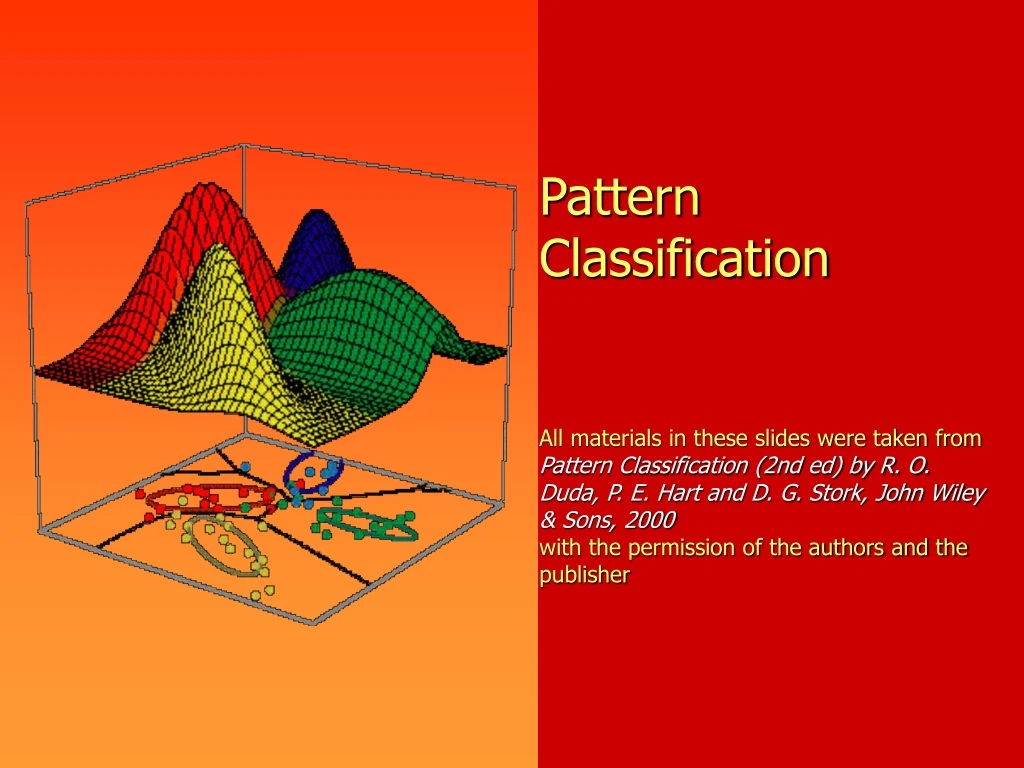
Pattern ClassificationAll materials in these slides were taken from Pattern Classification (2nd ed) by R. O. Duda, P. E. Hart and D. G. Stork, John Wiley & Sons, 2000with the permission of the authors and the publisher
Chapter 4: Nonparametric Techniques(Sections 1-6) Introduction Density Estimation Parzen Windows Kn–Nearest-Neighbor Estimation The Nearest-Neighbor Rule Metrics and Nearest-Neighbor Classification
1. Introduction • All Parametric densities are unimodal (have a single local maximum), whereas many practical problems involve multi-modal densities • Nonparametric procedures can be used with arbitrary distributions and without the assumption that the forms of the underlying densities are known • There are two types of nonparametric methods: • Estimate density functions P(x|j) without assuming a model • Parzen Windows • Bypass density functions and directly estimate P(j |x) • k-Nearest Neighbor (kNN) Pattern Classification, Ch4
2. Density Estimation Basic idea: • Probability that a vector x will fall in region R is: P is a smoothed version of the density function p(x) • For n samplesi.i.d. dist, probability that k points fall in R is: and the expected value for k is: E(k) = nP (3) Binomial distribution Pattern Classification, Ch4
Maximum Likelihood estimation of P = is reached for Therefore, the ratio k/n is a good estimate for the probability P and hence for the density function p. Because p(x) is continuous and the region R is so small that p does not vary significantly within it: where x is a point within R and V the volume enclosed by R. Pattern Classification, Ch4
Combining equations (1), (3), (4) => (5) 5 n = 20, 50, 100 Pattern Classification, Ch4
Theoretically, if an unlimited number of samples is available, we can estimate the density of x by forming a sequence of regions R1, R2,… containing x: the first contains one sample, the second two, etc. Let Vnbe the volume of Rn, kn the number of samples falling in Rn and pn(x) be the nth estimate for p(x): pn(x) = (kn/n)/Vn(7) Three conditions must apply for convergence : There are two different ways to satisfy these conditions:1. Shrink an initial region where Vn = 1/n and show that the Parzen-window estimation method 2. Specifykn as a function of n, such as kn = n; the volume Vnis grown until it encloses kn neighbors of x, the kNNestimation method Pattern Classification, Ch4
3. Parzen Windows • Parzen-window approach to estimate densities: assume e.g. that the region Rn is a d-dimensional hypercube • ((x-xi)/hn) is equal to unity if xi falls within the hypercube of volume Vn centered at x, and equal to zero otherwise. Pattern Classification, Ch4
The number of samples in this hypercube is: Substituting kn in equation 7 (pn(x) = (kn/n)/Vn) we obtain: Pn(x) estimates p(x) as an average of functions of x and the samples (xi) (i = 1,… ,n).These functions can be general! Pattern Classification, Ch4
Illustration – effect of window function • The behavior of the Parzen-window method • Case where p(x) N(0,1) Let (u) = (1/(2) exp(-u2/2) and hn = h1/n (n>1) (h1: parameter at our disposal) Thus: is an average of normal densities centered at the samples xi. Pattern Classification, Ch4
Numerical 1D results (see figure next slide): Results depend on n and h1 • For n = 1 and h1=1 • For n = 10 and h1= 0.1, the contributions of the individual samples are clearly observable ! Pattern Classification, Ch4
Case where p(x) = 1.U(a,b) + 2.T(c,d) (mixture of a uniform and a triangle density) Pattern Classification, Ch4
Classification example In classifiers based on Parzen-window estimation: • We estimate the densities P(x|j) for each category and classify a test point by the label corresponding to the maximum posterior (unequal priors for multiple classes can be included) • The decision region for a Parzen-window classifier depends upon the choice of window function as illustrated in the following figure. • For good estimates, usually n must be large, much greater than for parametric models Pattern Classification, Ch4
4. Kn–Nearest-Neighbor Estimation • Rather than trying to find the “best” Parzen window function • Let the cell volume be a function of the training data • Center a cell about x and let it grows until it captures knsamples (kn = f(n)) • knare called theknnearest-neighbors of x Two possibilities can occur: • Density is high near x so the cell will be small to provide good resolution • Density is low so the cell will grow until higher density regions are reached We can obtain a family of estimates by setting kn=k1/n and choosing different values for k1 (a parameter at our disposal)
Estimation of a-posteriori probabilities • Goal: estimate P(i | x) from a set of n labeled samples • Let’s place a cell of volume V around x and capture k samples • If kisamples among the k turned out to be labeled i , then: pn(x, i) = ki /n.V An estimate for pn(i| x) is:
ki/k is the fraction of the samples within the cell that are labeled i • For minimum error rate, the most frequently represented category within the cell is selected • If k is large and the cell sufficiently small, the performance will approach the best possible
5. The Nearest-Neighbor Rule • Let Dn = {x1, x2, …, xn} be a set of n labeled prototypes • Let x’ Dn be the closest prototype to a test point xthen the nearest-neighbor rule for classifying x is to assign it the label associated with x’ • The nearest-neighbor rule leads to an error rate greater than the minimum possible: the Bayes rate • If the number of prototypes is large (unlimited), the error rate of the nearest-neighbor classifier is never worse than twice the Bayes rate (it can be demonstrated!) • If n , it is always possible to find x’ sufficiently close so that: P(i | x’) P(i | x) • If P(m | x) 1, then the nearest neighbor selection is almost always the same as the Bayes selection
The k-nearest-neighbor rule • Goal: Classify x by assigning it the label most frequently represented among the k nearest samples and use a voting scheme • Usually choose k odd so no voting ties
Step-by-step algorithm for finding the nearest neighbor class decision regions and decision boundaries in 2D • Find the midpoints between all pairs of points. • Find the perpendicular bisectorsof the lines between all pairs of points (they go through the midpoints found in step 1). • Find the point regions, the region surrounding each point that is closest to the point (this region is outlined by the perpendicular bisector segments that are perpendicular to the shortest line from the point to the bisector segment). These regions are called Voronoicells. • Merge adjoining point regions of the same class (such as a two-class problem of dog versus cat) to obtain class decision regions(any point falling into the region is assigned to the class of the region). This is done by eliminating the boundary lines (perpendicular bisector segments) between points of the same class. The resulting connected line segments defining the decision regions are called the decision boundaries.
Example: k = 3 (odd value) and x = (0.10, 0.25)t Closest vectors to x with their labels are: {(0.10, 0.28, 2); (0.12, 0.20, 2); (0.15, 0.35,1)} One voting scheme assigns the label 2 to x since 2 is the most frequently represented
6. Metrics and Nearest-Neighbor Classification • kNN uses a metric (distance function) between two vectors • Typically Euclidean distance • Distance functions have the properties of
The MinkowskiMetric or Distance • L1 is the Manhattan or city block distance • L2 is the Euclidean distance