Download
1 / 23
230 likes | 439 Views
Dynamic causal modelling of electromagnetic responses Karl Friston - Wellcome Trust Centre for Neuroimaging, Institute of Neurology, UCL

E N D
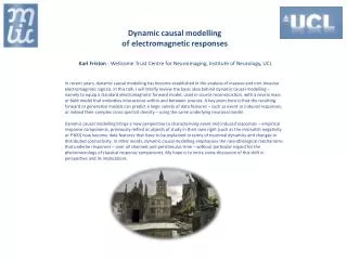
Dynamic causal modelling of electromagnetic responses Karl Friston - Wellcome Trust Centre for Neuroimaging, Institute of Neurology, UCL In recent years, dynamic causal modelling has become established in the analysis of invasive and non-invasive electromagnetic signals. In this talk, I will briefly review the basic idea behind dynamic causal modelling – namely to equip a standard electromagnetic forward model, used in source reconstruction, with a neural mass or field model that embodies interactions within and between sources. A key point here is that the resulting forward or generative models can predict a large variety of data features – such as event or induced responses, or indeed their complex cross spectral density – using the same underlying neuronal model. Dynamic causal modelling brings a new perspective to characterising event and induced responses – empirical response components, previously reified as objects of study in their own right (such as the mismatch negativity or P300) now become data features that have to be explained in terms of neuronal dynamics and changes in distributed connectivity. In other words, dynamic causal modelling emphasises the neurobiological mechanisms that underlie responses – over all channels and peristimulus time – without particular regard for the phenomenology of classical response components. My hope is to incite some discussion of this shift in perspective and its implications.
One ring to rule them all, one ring to find them, one ring to bring them all, and in the darkness bind them
Overview The basic idea (functional and effective connectivity) Generative model and face validation An empirical example
Exogenous and endogenous fluctuations Generative model Neuronal dynamics Evoked responses Induced responses
Exogenous and endogenous fluctuations Model inversion
Bayesian model inversion and parameter averaging Invert model of evoked responses We seek the posterior conditioned on both evoked and induced responses. Using Bayes rule we have: Update priors Invert model of induced responses Giving the likelihood and prior for induced responses Inference on parameters and models
Models of effective connectivity among hidden states causing observed responses State-space model Convolution kernel representation Functional Taylor expansion Spectral representation Convolution theorem Autoregressive representation Yule Walker equations Spectral representation Convolution theorem Cross-covariance Auto-regression coefficients Cross-spectral density Directed transfer functions Cross-correlation Coherence Auto-correlation Granger causality Measures of functional connectivity or statistical dependence among observed responses
Effective connectivity Modulation transfer functions Volterra kernels Cross covariance functions Cross spectral density Spectral measures Auto regression coefficients Spectral factors Director transfer functions Granger causality parametric nonparametric
Overview The basic idea Generative model and face validation An empirical example
Generative (conductance based neural mass) model based on the canonical microcircuit Inhibitory connections: k = E Excitatory connections: k = I Superficial pyramidal cells Forward extrinsic connections Inhibitory interneurons supragranular layer Spiny stellate cells Granular layer Intrinsic connections Infragranular layer Backward extrinsic connections Deep pyramidal cells Exogenous (subcortical) input Endogenous fluctuations Endogenous fluctuations Higher source (2) Early source (1)
The effect of parameters on transfer functions – contribution analysis Intrinsic backward connections) Transfer functions 4 60 50 3 40 Frequency 2 30 20 1 10 0 0 10 20 30 40 50 60 70 -2 -1 0 1 2 (log) parameter scaling frequency {Hz} 32 8 1 2 32 8 4 4 8 4 Self-inhibition of superficial cells Transfer functions 5 60 4 50 3 40 Frequency 30 2 20 1 10 0 0 10 20 30 40 50 60 70 -2 -1 0 1 2 (log) parameter scaling frequency {Hz}
Predicted responses to sustained exogenous (stimulus) input Evoked response: source 1 Induced response 8 6 60 Exogenous input 6 4 50 4 40 2 Hz 2 30 0 0 20 50 100 150 200 250 300 350 400 450 500 -2 peristimulus time (ms) 10 100 200 300 400 500 100 200 300 400 500 Hidden neuronal states (conductance and depolarisation) peristimulus time (ms) peristimulus time (ms) Evoked response: source 2 Induced response 0 60 -20 4 50 -40 2 40 Hz -60 0 30 50 100 150 200 250 300 350 400 450 500 source 2 source 1 -2 20 peristimulus time (ms) 10 -4 100 200 300 400 500 100 200 300 400 500 peristimulus time (ms) peristimulus time (ms) Spectral density Coherence 60 60 50 50 40 40 Hz Hz 30 30 20 20 10 10 100 200 300 400 500 100 200 300 400 500 peristimulus time (ms) peristimulus time (ms) Cross-covariance Spectral density 60 60 40 50 20 40 lag (ms) Hz 0 30 -20 20 -40 10 -60 100 200 300 400 500 100 200 300 400 500 peristimulus (ms) peristimulus time (ms)
Transfer functions and spectral asymmetries Forward connections (gamma) backward connections (beta) Endogenous fluctuations Endogenous fluctuations
Spectral density Coherence evoked: source 1 Simulated responses (sample estimates over16 trials) 60 60 6 50 50 4 40 40 2 Hz Hz 30 30 0 20 20 -2 10 10 -4 100 200 300 400 500 100 200 300 400 500 100 200 300 400 500 peristimulus time (ms) peristimulus time (ms) peristimulus time (ms) Cross-covariance Spectral density evoked: source 2 60 50 5 50 40 0 lag (ms) Hz 0 30 20 -5 -50 10 100 200 300 400 500 100 200 300 400 500 100 200 300 400 500 peristimulus (ms) peristimulus time (ms) peristimulus time (ms) evoked: source 1 Spectral density Coherence Predicted responses (expectation under known input) 6 60 60 4 50 50 40 40 2 Hz Hz 30 30 0 20 20 -2 10 10 100 200 300 400 500 100 200 300 400 500 100 200 300 400 500 peristimulus time (ms) peristimulus time (ms) peristimulus time (ms) evoked: source 2 Cross-covariance Spectral density 60 50 4 50 2 40 lag (ms) Hz 0 0 30 -2 20 -50 10 -4 100 200 300 400 500 100 200 300 400 500 100 200 300 400 500 peristimulus time (ms) peristimulus (ms) peristimulus time (ms)
Overview The basic idea Generative model and face validation An empirical example
Functional asymmetries in forward and backward connections Phenomenological DCM for induced responses (Chen et al 2008) FLBL FNBL FLBN FNBN 4 12 20 28 36 44 0 -10000 Frequency (Hz) 44 36 28 20 12 4 -20000 SPM t -30000 -40000 -50000 From 32 Hz (gamma) to 10 Hz (alpha) t = 4.72; p = 0.002 -60000 -70000 0.1 0.1 0.08 0.08 RF LF 0.06 0.06 0.04 0.04 0.02 0.02 0 0 LV RV -0.02 -0.02 -0.04 -0.04 Forward Backward Forward Backward -0.06 -0.06 -0.08 -0.08 input -0.1 -0.1 Left hemisphere Right hemisphere
Posterior predictions following inversion of event responses Sensor level observations Estimates of dipole orientation Predicted Observed (adjusted) 1 -100 -100 0 0 100 100 time (ms) time (ms) 200 200 300 300 400 400 500 500 50 100 150 200 250 50 100 150 200 250 RF LF channels channels LV RV and DCM predictions input
Posterior predictions following inversion of induced responses
Transfer functions and spectral asymmetries transfer function: 1 to 1 transfer function: 3 to 1 30 30 Hz Hz 20 20 10 10 0 200 400 0 200 400 peristimulus time (ms) peristimulus time (ms) transfer function: 1 to 3 transfer function: 3 to 3 Forward connections (gamma?) Backward connections (beta) 30 30 Hz Hz 20 20 10 10 0 200 400 0 200 400 peristimulus time (ms) peristimulus time (ms) kernel: 1 to 1 kernel: 3 to 1 0.5 2 0 0 -0.5 -2 0 100 0 100 lag (ms) lag (ms) RF RF LF LF kernel: 1 to 3 kernel: 3 to 3 10 0.5 LV LV RV RV 0 0 -10 -0.5 0 100 0 100 lag (ms) lag (ms) input input
Thank you And thanks to Gareth Barnes Andre Bastos CC Chen Jean Daunizeau Marta Garrido Lee Harrison Martin Havlicek Stefan Kiebel Marco Leite Vladimir Litvak Andre Marreiros Rosalyn Moran Will Penny Dimitris Pinotsis Krish Singh Klaas Stephan Bernadette van Wijk And many others
Errors (superficial pyramidal cells) Forward transfer function 14 12 10 Expectations (deep pyramidal cells) 8 spectral power 6 Andre Bastos 4 2 0 0 20 40 60 80 100 V4 V1 0.3 0.25 0.2 superficial 0.15 0.1 0.05 0 0 20 40 60 80 100 120 6 5 4 spectral power 3 2 2 1 deep 0 0 20 40 60 80 100 1 frequency (Hz) Backward transfer function 0 0 20 40 60 80 100 120 frequency (Hz)