Download
1 / 41
410 likes | 538 Views
Getting optimal load distribution using transport-problem-based algorithm. Y.V. Ladyzhensky , V.A. Kourktchi Donetsk National Technical University, TODC, LLC. Dynamic Load Balancing. Given: The set V P of P processors each process l i subproblems

E N D
Getting optimal load distribution using transport-problem-based algorithm Y.V. Ladyzhensky, V.A. Kourktchi Donetsk National Technical University, TODC, LLC
Dynamic Load Balancing Given: • The set VP of P processors each process li subproblems • The processor graph GP(VP,EP) with edge (i, j)EP if data can be transferred from a processor i to a processor j • The problem graph GN(VN,EN):VN is the set of subproblems; EN is the set of edges. An edge (i, j)EN if the subproblem j needs information or events from the subproblem i.
Dynamic Load Balancing Find new allocation of subproblems to the processors: • The maximum load li should be minimal • The number of migrated subproblems should be minimal
Distributed Logic Simulation Properties: • Since the computing network is used the problem graph is full • Since the network communications are slow criteria of data migration is crucial.
Transport-Problem-Based Algorithm Stages: • Find all shortest paths in the processors graph using Floyd algorithm • Find processors with surplus load • Find processors with lack of load • Form input data for the method of potential • Solve the transportation problem • Move the subproblems using gained migration schedule
Transport-Problem-Based Algorithm Stages: • Find all shortest paths in the processors graph using Floyd algorithm • Find processors with surplus load • Find processors with lack of load • Form input data for the method of potential • Solve the transportation problem • Move the subproblems using gained migration schedule
¬ D,W Floyd(G(C, E )) N Transport-Problem-Based Algorithm Results of Floyd algorithm: • Matrix D represents the lengths of ways • Matrix W information about ways
Transport-Problem-Based Algorithm Stages: • Find all shortest paths in the processors graph using Floyd algorithm • Find processors with surplus load • Find processors with lack of load • Form input data for the method of potential • Solve the transportation problem • Move the subproblems using gained migration schedule
¬ - ³ 1 O {C ||C | l } i i avg é ù P 1 å = l C ê ú avg i P ê ú = i 1 Transport-Problem-Based Algorithm The set Ocontains processors with surplus load
Transport-Problem-Based Algorithm Stages: • Find all shortest paths in the processors graph using Floyd algorithm • Find processors with surplus load • Find processors with lack of load • Form input data for the method of potential • Solve the transportation problem • Move the subproblems using gained migration schedule
¬ < } I {C ||C | l i i avg é ù P 1 å = l C ê ú avg i P ê ú = i 1 Transport-Problem-Based Algorithm The set Icontains processors with lack of load
Transport-Problem-Based Algorithm Stages: • Find all shortest paths in the processors graph using Floyd algorithm • Find processors with surplus load • Find processors with lack of load • Form input data for the method of potential • Solve the transportation problem • Move the subproblems using gained migration schedule
O1 = Ci1 O2 = Ci2 Om=Cim I1=Cj1 I2=Cj2 Ik=Cjk Transport-Problem-Based Algorithm Di1j1 Di1j2 Di1jk Di2j1 Di2j2 Di2jk Dimj1 Dimj2 Dimjk
Transport-Problem-Based Algorithm Stages: • Find all shortest paths in the processors graph using Floyd algorithm • Find processors with surplus load • Find processors with lack of load • Form input data for the method of potential • Solve the transportation problem • Move the subproblems using gained migration schedule
Transport-Problem-Based Algorithm • Potentials method results example • Move 5 subproblems from processor 3 to processor1 • Way length is 2 which means 1 transit processor will be used
Transport-Problem-Based Algorithm Stages: • Find all shortest paths in the processors graph using Floyd algorithm • Find processors with surplus load • Find processors with lack of load • Form input data for the method of potential • Solve the transportation problem • Move the subproblems using gained migration schedule
Î foreach k O Î foreach m I c:=vs repeat D ¬ D [c,W[c,m]] [c,W[c,m]] +TS[k,m] ¬ c W[c,m]; until c=m; endfor endfor Transport-Problem-Based Algorithm
Transport-Problem-Based Algorithm • Use matrix W to restore paths between each pair of processors belonging to the sets O and I • The result of transportation problem is added to each edge on the path fromOi toIj
Advantages • Potential methods guarantees the minimum level of migration.
Disadvantage • For some input data the misbalance can be significant after balancing.
Disadvantage • Example: 381 subproblems,20 processors
é ù P 1 å = l C ê ú avg i P ê ú = i 1 ê ú P 1 å = l C ê ú avg i P ë û = i 1 Getting optimal balance • Use algorithm considering average load as • Reuse algorithm considering average load as
Before balancing 362 1 1 1 1 1 1 1 1 1 1 1 1 1 1 1 1 1 1 1 After balancing 20 20 20 20 20 20 20 20 20 20 20 20 20 20 20 20 20 20 20 1 After secondary balancing 20 19 19 19 19 19 19 19 19 19 19 19 19 19 19 19 19 19 19 19 Optimal solution 20 19 19 19 19 19 19 19 19 19 19 19 19 19 19 19 19 19 19 19 Getting optimal balance • Example
Getting optimal balance • The possibility to get optimal balance for any input data has been proved.
Algorithms Testing (misbalance) 10000 subproblems, 20 processors
Algorithms Testing (migration level) 10000 subproblems, 20 processors
Algorithms Testing (migration level) 10000 subproblems, 20 processors
Conclusion • Algorithm that guarantee optimal subproblem distribution from the misbalance point of view is developed. • Migration level non significantly increases in comparison with original Transport-problem based algorithm and still 20% lower than Hu-Blake method.
Future research • Improve the transport-problem-based algorithm by taking in account communications between subproblems • Lower migration to minimum level.
Transport-Problem-Based Algorithm Work example: • Input data: 6 vertices process graph 180 subproblems • Subproblems allocation 10, 40, 55, 20, 20, 35 • Average load is 30 subproblems
Transport-Problem-Based Algorithm Work example: • Result of Floyd algorithm
Transport-Problem-Based Algorithm Work example: • Surplus load: • processor 2 – 10 surplus subproblems • processor 3 – 25 surplus subproblems • Processor 6 – 5 surplus subproblems
Transport-Problem-Based Algorithm Work example: • Surplus load: • processor 1 – 20 deficit subproblems • processor 4 – 10 deficit subproblems • Processor 5 – 10 deficit subproblems
Transport-Problem-Based Algorithm Work example: • Input data for method of potentials
10 0 1 1 2 - + 10 10 5 1 2 1 1 + - 5 1 1 2 3 1 0 0 Transport-Problem-Based Algorithm Work example: • Initial solution (using the north-west corner method) • Calculate potentials • Find cycle
Transport-Problem-Based Algorithm Work example: • New solution • This solution is optimal
Transport-Problem-Based Algorithm Work example: • Move 10 subproblems from processor 2 to processor 1 • Move 5 subproblems from processor 3 to processor 1 • Move 10 subproblems from processor 3 to processor 4 • Move 10 subproblems from processor 3 to processor 5 • Move 5 subproblems from processor 6 to processor 1
Transport-Problem-Based Algorithm Work example: • The processors 3 and 1 are not connected • Move 5 subproblems from processor 3 to processor 2 • Then move 5 subproblems from processor 2 to processor 1
Transport-Problem-Based Algorithm Work example: • Migration schedule • Move 10+10+10+5+ +5+5 subproblems
Transport-Problem-Based Algorithm Work example: • Result: new load allocation • Allocation is optimal • 45 subproblems moved