Download
1 / 47
530 likes | 618 Views
Social Ties and Link Prediction. Kristina Lerman University of Southern California. Link Prediction. Will nodes 33 and 28 become friends in the future?. Does network structure contain enough information to predict what new links will form in the future?. What about nodes 27 and 4?.

E N D
Social Ties and Link Prediction Kristina Lerman University of Southern California CS 599: Social Media Analysis University of Southern California
Link Prediction Will nodes 33 and 28 become friends in the future? Does network structure contain enough information to predict what new links will form in the future? What about nodes 27 and 4?
Strength of social ties (review) • Strong ties • surrounded by many mutual friends • characterized by lots of shared time together • Weak ties • have few mutual friends • Serve as bridges to diverse parts of the network • Provide access to novel information
The Link-Prediction Problem for Social Networks (Liben-Nowell & Kleinberg) To what extent can the evolution of a social network be modeled using features intrinsic to the network itself? • Formalize the link prediction problem • Given a snapshot of a network, infer which new interactions between nodes are likely to occur in the future • Propose link prediction heuristics based on measures for analyzing the “proximity” of nodes in a network. • Evaluate link prediction heuristics on large coauthorshipnetworks. Future coauthorshipscan be extracted from network topology.
The intuition • In many networks, people who are “close” belong to the same social circles and will inevitably encounter one another and become linked themselves. • Link prediction heuristics measure how “close” people are x x y y Red nodes are more distant Red nodes are close to each other
Link prediction heuristics • Local • Common neighbors (CN) • Jaccard (JC) • Adamic-Adar (AA) • Preferential attachment (PA) … • Global • Katz score • Hitting time • PageRank … x y
Local link prediction heuristics • Link prediction heuristics • Common neighbors (CN) • Neighborhood overlap • Jaccard (JC) • Adamic-Adar (AA) • Preferential attachment (PA) x y
Local link prediction heuristics • Link prediction heuristics • Common neighbors (CN) • Jaccard (JC) • Fraction of common neighbors • Adamic-Adar (AA) • Preferential attachment (PA) x y
Link prediction heuristics • Link prediction heuristics • Common neighbors (CN) • Jaccard (JC) • Adamic-Adar (AA) • Nmbr common neighbors, with each neighbor z attenuated by log of its degree • Preferential attachment (PA) x y
Local link prediction heuristics • Link prediction heuristics • Common neighbors (CN) • Jaccard (JC) • Adamic-Adar (AA) • Preferential attachment (PA) • Better connected nodes are more likely to form more links x y
Global link prediction heuristics • Link prediction heuristics • Katz score • Measures number of paths between two nodes, attenuated by their length • Hitting time • Expected time for a random walk from x to reach y • … x y
Data • Collaboration networks of physicists • Core nodes: authors who published at least 3 papers during the training period and at least 3 papers during test period • Training data: graph G(t0, t0’) of collaborations during time period [t0, t0‘] with V core nodes and Eold edges • Test data: graph G(t1, t1’) of collaborations during a later time period [t1, t1’] with V core nodes and Enew edges
Evaluation metric • Link prediction algorithm • Score node pairs using a heuristic p • New links more likely among high scoring pairs • Each link prediction heuristic p outputs a ranked list L of new collaborations: pairs in VxV-Eold. • Focus evaluation on new links Enew* between core nodes • Performance metric: How many of the top n pairs in ranked list L are the actual new nodes in Enew*?
Results Heuristics vs random predictor
Results Heuristics vs graph distance predictor
Summary • Graph-based link prediction heuristics outperform random guess by a factor of 40 • However, they still predict only 16% of new collaborations at best, leaving much room for improvement.
CSCI 599 Social Media Analysis Link prediction in complex networks: a survey Presenter: Yuan Shi USC ID: 7678039433 L Lu and T Zhou, “Link prediction in complex networks: a survey”, Physica A 390(6):11501170 (2011)
Link Prediction • Estimate the likelihood of the existence of a link between two nodes, based on observed linksand the attributes of nodes • Application • Biological networks: costly to identify links between nodes through field/laboratorial experiments • Online social networks: predicting friendship and recommending new friends (predicting future links in evolving networks)
Problem Description and Evaluation Metrics • Undirected network G = (V, E) • Universal set U containing |V|(|V|-1)/2 possible links • Task: Find out missing links in U – E. • Evaluation: randomly split E into two sets: training set ET , probe/validation set EP • k-folder cross validation • Randomly partition into k subsets • Each time one subset is selected as probe set, the others as training set • Repeat k times, each with a different probe set
Evaluation Metrics • A link prediction algorithm gives a ranking on each link • AUC (area under the receiver operating characteristic curve) • Focus the whole list of ranks • The probability that a randomly chosen missing link is given a higher score than a randomly chosen nonexistent link • Precision • Focus on the top ranks • Take top-L predicted links, among which Lr links are right, the precision is Lr/L
Similarity-Based Algorithms • Assign a score sxy to each pair of nodes x and y • The attributes of nodes are generally hidden -> focus on structural similarity: two nodes are linked if they have similar network structure • Similarity indices • Local similarity Indices: only use local information • Global similarity indices: use global information, more accurate but costly • Quasi-local indices: a tradeoff between local and global
Local similarity Indices • 10 indices are discussed. • Common neighbors (CN) • Resource Allocation Index (RA) • Adamic-Adar Index (AA) set of neighbors degree of note z • Intuition: • Similarity(x, y) = the amount of resource y received from x • x sends some resource to y, with their common neighbors as transmitters • Each transmitter has a unit of resource and will equally distribute it to all its neighbors
Local similarity Indices - Evaluation Metric: AUC. Each number averaged by 10 implementations. Real-world networks PPI: protein-protein interaction NS: co-authorship Grid: electrical power-grid PB: US political blogs INT: router-level Internet USAir: US air transportation CN and AA have second best performance RA performs the best
Global similarity Indices • 7 indices are discussed. Some examples are: • Katz Index • Average Commute Time • Random Walk with Restart (direct application of PageRank algorithm) • Global indices • Pros: more accurate than local indices • Cons: 1) time-consuming; 2) global topological information may not be available Laplacian matrix
Quasi-local Indices • 3 indices are discussed. • Local Path Index (LP) • Outperforms local indices like RA, AA and CN • Performs competitively to global indices with much less computational cost • Local Random Walk (LRW): at time step t, • Superposed Random Walk (SRW): at time step t, q is initial configuration function, e.g. Some experiments show LRW and SRW performs better than LP
Maximum Likelihood Methods • Methodology • Assume some organizing principles of the network structure • Rules and parameters are obtained by maximizing the likelihood of the observed structure • Likelihood of any non-observed link can be calculated according to those rules and parameters • Pros: provide valuable insights into the network organization • Cons: Time consuming; Prediction accuracy is not very high
Example: Hierarchical Structure Model Assumption: 1. Each internal node r associated with a probability pr 2. Probability of linking a pair of leaves equals to pr’ where r’ is their lowest common ancestor Some statistics of the graph By maximizing the likelihood, Prediction: 1. Sample a large number of dendrograms with probability proportional to their likelihood 2. Compute the link probability by averaging the corresponding probability over all sampled dendrograms
Application • Reconstruction of Networks • Not easy to reconstruct the “true” network since generally no one knows how many links are missing • Reliability of a network • Classification of Partially Labeled Networks • Predict the labels of these unlabeled nodes based on the known labels and the network structure • Approach: add artificial links between every pair of labeled and unlabeled nodes Global optimization is difficult -> use greedy algorithms
Application • Evaluation of Network Evolving Mechanisms • link prediction algorithm tells the factors resulting in the existence of links • Example: Similarity indices for the Chinese city airline network CN: topological effects DIS: geographical distance POPU: population GDP TI: third sector of GDP, named the tertiary industry
Outlook • Link prediction in directed networks • Multi-dimensional networks, where links could have different meanings (e.g. positive/negative) • Hybrid algorithms to combine different similarity indices • Leveraging external information (e.g. attributes) to improve accuracy • Time-series link prediction approach considering the temporal evolutions of link occurrences
Romantic Partnerships and the Dispersion of Social Ties (Backstrom & Kleinberg) • Questions • Who are the most important individuals in a person’s social neighborhood? • What are the defining structural signatures of a person’s social neighborhood? • Contributions • Dispersion: a new measure for estimating tie strength • Characterize romantic relationships in terms of network structure • Empirical study of this characteristic across Facebook population
Who are the most important people in one’s social neighborhood? • Following Granovetter, researchers use number of mutual friends (embeddedness) to identify strong ties • Close friends, who share much time together • Emotionally intense interactions A-B tie is highly embedded in the network A-B tie is not embedded in the network C C A A D D E E B B F F
Romantic ties • Embeddedness is not able to identify “significant others” (romantic relationships, e.g., spouse, partner, boy/girlfriend) • Ego network – social neighborhood of an individual, showing all his/her friends and links between them Who is the “significant other”? Ego network of an individual
Social foci • People have large clusters of friends corresponding to well-defined foci of interaction in their lives • These links have high embeddedness but are not very strong ties • In contrast, romantic partners may have lower embeddedness, but they often involve mutual friends from different foci Co-workers Ego network of an individual College friends
Embeddedness vs dispersion Dispersion: mutual neighbors of u and v are not well-connected to one another, and hence u and v are the only intermediaries between these different parts of the network. Link u-h has high dispersion: u and h are the only intermediaries between c and f Embeddedness: u and v have many mutual neighbors. Links u-b, u-c, and u-f have embeddedness 5 Link u-h has embeddedness 4
Link dispersion disp(u,b)=1 s(u,h)=4
Evaluation • Egonetworks of 1.3 million Facebook users, selected uniformly at random from among all users of age at least 20, with between 50 and 2000 friends, who list a spouse or relationship partner in their profile • Rank all friends by importance. Attempt to identify romantic partners • Measure: Precision of the first position, Pr@1
Performance – Pr@1 • How well does dispersion predict the “significant other”? – precision of the top-ranked person in the individual’s egonet • Beats others measures of interaction between users • viewing of profiles, sending of messages, and co-presence at events (photos)
Performance as a function of neighborhood size • Performance is best when the neighborhood size is around 100 nodes (56%), & drops moderately (to 33%) as the egonet size increases by an order of magnitude to 1000 • Interaction features are better for larger neighborhoods, due to users with larger neighborhoods being more active
Best performance when combining features • Predict relationship status of users • Ground truth: 60% of users are in a relationship • Demographic features (age, gender, country, and time on site) work better than network-based features (dispersion) • Best performance combining demographic and network features
Marriage • Performance of dispersion measures increases as people approach time of their marriage
Persistence of relationships • Transition probability from the status ‘in a relationship’ to the status ‘single’ over a 60-day period. The transition probabilities decrease monotonically, and by significant factors, for users with high normalized or recursive dispersion to their respective partners.
Summary • Graph structure contains information predictive of individual relationships • New collaborations • Romantic partnerships • In many cases, graph-based algorithms outperform feature-based machine learning algorithms • These suggest complex interactions between personal relationships and global network structure