Image Features: Descriptors and matching

1. Image Features:Descriptors and matching CSE 576, Spring 2005 Richard Szeliski

2. Today’s lecture • Feature detectors • scale and affine invariant (points, regions) • Feature descriptors • patches, oriented patches • SIFT (orientations) • Feature matching • exhaustive search • hashing • nearest neighbor techniques CSE 576: Computer Vision

3. Pointers to papers: CSE 576: Computer Vision

4. Invariant Local Features • Image content is transformed into local feature coordinates that are invariant to translation, rotation, scale, and other imaging parameters SIFT Features CSE 576: Computer Vision

5. Advantages of local features • Locality: features are local, so robust to occlusion and clutter (no prior segmentation) • Distinctiveness: individual features can be matched to a large database of objects • Quantity: many features can be generated for even small objects • Efficiency: close to real-time performance • Extensibility: can easily be extended to wide range of differing feature types, with each adding robustness CSE 576: Computer Vision

6. Scale Invariant Detection • Consider regions (e.g. circles) of different sizes around a point • Regions of corresponding sizes will look the same in both images CSE 576: Computer Vision

7. Scale Invariant Detection • The problem: how do we choose corresponding circles independently in each image? CSE 576: Computer Vision

8. Scale invariance • Requires a method to repeatably select points in location and scale: • The only reasonable scale-space kernel is a Gaussian (Koenderink, 1984; Lindeberg, 1994) • An efficient choice is to detect peaks in the difference of Gaussian pyramid (Burt & Adelson, 1983; Crowley & Parker, 1984 – but examining more scales) • Difference-of-Gaussian with constant ratio of scales is a close approximation to Lindeberg’s scale-normalized Laplacian (can be shown from the heat diffusion equation) CSE 576: Computer Vision

9. scale = 1/2 Image 1 f f Image 2 region size region size Scale Invariant Detection • Solution: • Design a function on the region (circle), which is “scale invariant” (the same for corresponding regions, even if they are at different scales) Example: average intensity. For corresponding regions (even of different sizes) it will be the same. • For a point in one image, we can consider it as a function of region size (circle radius) CSE 576: Computer Vision

10. scale = 1/2 Image 1 f f Image 2 s1 s2 region size region size Scale Invariant Detection • Common approach: Take a local maximum of this function Observation: region size, for which the maximum is achieved, should be invariant to image scale. Important: this scale invariant region size is found in each image independently! CSE 576: Computer Vision

11. f f Good ! bad region size f region size bad region size Scale Invariant Detection • A “good” function for scale detection: has one stable sharp peak • For usual images: a good function would be a one which responds to contrast (sharp local intensity change) CSE 576: Computer Vision

12. Scale Invariant Detection • Functions for determining scale Kernels: (Laplacian) (Difference of Gaussians) where Gaussian Note: both kernels are invariant to scale and rotation CSE 576: Computer Vision

13. Scale space: one octave at a time CSE 576: Computer Vision

14. Key point localization • Detect maxima and minima of difference-of-Gaussian in scale space • Fit a quadratic to surrounding values for sub-pixel and sub-scale interpolation (Brown & Lowe, 2002) • Taylor expansion around point: • Offset of extremum (use finite differences for derivatives): CSE 576: Computer Vision

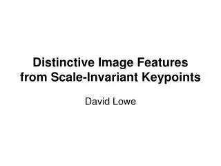
15. scale  Laplacian  y x  Harris  scale • SIFT (Lowe)2Find local maximum of: • Difference of Gaussians in space and scale  DoG  y x  DoG  Scale Invariant Detectors • Harris-Laplacian1Find local maximum of: • Harris corner detector in space (image coordinates) • Laplacian in scale 1 K.Mikolajczyk, C.Schmid. “Indexing Based on Scale Invariant Interest Points”. ICCV 20012 D.Lowe. “Distinctive Image Features from Scale-Invariant Keypoints”. Accepted to IJCV 2004 CSE 576: Computer Vision

16. Scale Invariant Detection: Summary • Given:two images of the same scene with a large scale difference between them • Goal:find the same interest points independently in each image • Solution: search for maxima of suitable functions in scale and in space (over the image) • Methods: • Harris-Laplacian [Mikolajczyk, Schmid]: maximize Laplacian over scale, Harris’ measure of corner response over the image • SIFT [Lowe]: maximize Difference of Gaussians over scale and space CSE 576: Computer Vision

17. Affine invariant detection • Above we considered:Similarity transform (rotation + uniform scale) • Now we go on to:Affine transform (rotation + non-uniform scale) CSE 576: Computer Vision

18. Affine invariant detection • Harris-Affine [Mikolajczyk & Schmid, IJCV04]: • use Harris moment matrix to select dominant directions and anisotropy CSE 576: Computer Vision

19. Affine invariant detection • Matching Widely Separated Views Based on Affine Invariant Regions, T. TUYTELAARS and L. VAN GOOL, IJCV 2004 CSE 576: Computer Vision

20. f points along the ray Affine invariant detection • Take a local intensity extremum as initial point • Go along every ray starting from this point and stop when extremum of function f is reached • We will obtain approximately corresponding regions Remark: we search for scale in every direction CSE 576: Computer Vision

21. Geometric Moments: Fact: moments mpq uniquely determine the function f Taking f to be the characteristic function of a region (1 inside, 0 outside), moments of orders up to 2 allow to approximate the region by an ellipse This ellipse will have the same moments of orders up to 2 as the original region Affine invariant detection • The regions found may not exactly correspond, so we approximate them with ellipses CSE 576: Computer Vision

22. ( p = [x, y]T is relative to the center of mass) Affine invariant detection • Covariance matrix of region points defines an ellipse: Ellipses, computed for corresponding regions, also correspond CSE 576: Computer Vision

23. Affine invariant detection • Algorithm summary (detection of affine invariant region): • Start from a local intensity extremum point • Go in every direction until the point of extremum of some function f • Curve connecting the points is the region boundary • Compute geometric moments of orders up to 2 for this region • Replace the region with ellipse CSE 576: Computer Vision

24. MSER J.Matas et.al. “Distinguished Regions for Wide-baseline Stereo”. BMVC 2002. • Maximally Stable Extremal Regions • Threshold image intensities: I > I0 • Extract connected components(“Extremal Regions”) • Find a threshold when an extremalregion is “Maximally Stable”,i.e. local minimum of the relativegrowth of its square • Approximate a region with an ellipse CSE 576: Computer Vision

25. Affine invariant detection • Under affine transformation, we do not know in advance shapes of the corresponding regions • Ellipse given by geometric covariance matrix of a region robustly approximates this region • For corresponding regions ellipses also correspond • Methods: • Search for extremum along rays [Tuytelaars, Van Gool]: • Maximally Stable Extremal Regions [Matas et.al.] CSE 576: Computer Vision

26. Today’s lecture • Feature detectors • scale and affine invariant (points, regions) • Feature descriptors • patches, oriented patches • SIFT (orientations) • Feature matching • exhaustive search • hashing • nearest neighbor techniques CSE 576: Computer Vision

27. Feature selection • Distribute points evenly over the image CSE 576: Computer Vision

28. Adaptive Non-maximal Suppression • Desired: Fixed # of features per image • Want evenly distributed spatially… • Search over non-maximal suppression radius[Brown, Szeliski, Winder, CVPR’05] r = 8, n = 1388 r = 20, n = 283 CSE 576: Computer Vision

29. Feature descriptors • We know how to detect points • Next question: How to match them? ? • Point descriptor should be: • Invariant 2. Distinctive CSE 576: Computer Vision

30. Descriptors invariant to rotation • Harris corner response measure:depends only on the eigenvalues of the matrix M • Careful with window effects! (Use circular) CSE 576: Computer Vision

31. Multi-Scale Oriented Patches • Interest points • Multi-scale Harris corners • Orientation from blurred gradient • Geometrically invariant to similarity transforms • Descriptor vector • Bias/gain normalized sampling of local patch (8x8) • Photometrically invariant to affine changes in intensity • [Brown, Szeliski, Winder, CVPR’2005] CSE 576: Computer Vision

32. Descriptor Vector • Orientation = blurred gradient • Similarity Invariant Frame • Scale-space position (x, y, s) + orientation () CSE 576: Computer Vision

33. MOPS descriptor vector • 8x8 oriented patch • Sampled at 5 x scale • Bias/gain normalisation: I’ = (I – )/ 40 pixels 8 pixels CSE 576: Computer Vision

34. SIFT vector formation • Thresholded image gradients are sampled over 16x16 array of locations in scale space • Create array of orientation histograms • 8 orientations x 4x4 histogram array = 128 dimensions CSE 576: Computer Vision

35. SIFT – Scale Invariant Feature Transform1 • Empirically found2 to show very good performance, invariant to image rotation, scale, intensity change, and to moderate affine transformations Scale = 2.5Rotation = 450 1 D.Lowe. “Distinctive Image Features from Scale-Invariant Keypoints”. Accepted to IJCV 20042 K.Mikolajczyk, C.Schmid. “A Performance Evaluation of Local Descriptors”. CVPR 2003 CSE 576: Computer Vision

36. Invariance to Intensity Change • Detectors • mostly invariant to affine (linear) change in image intensity, because we are searching for maxima • Descriptors • Some are based on derivatives => invariant to intensity shift • Some are normalized to tolerate intensity scale • Generic method: pre-normalize intensity of a region (eliminate shift and scale) CSE 576: Computer Vision

37. Today’s lecture • Feature detectors • scale and affine invariant (points, regions) • Feature descriptors • patches, oriented patches • SIFT (orientations) • Feature matching • exhaustive search • hashing • nearest neighbor techniques CSE 576: Computer Vision

38. Feature matching • Exhaustive search • for each feature in one image, look at all the other features in the other image(s) • Hashing • compute a short descriptor from each feature vector, or hash longer descriptors (randomly) • Nearest neighbor techniques • k-trees and their variants (Best Bin First) CSE 576: Computer Vision

39. Wavelet-based hashing • Compute a short (3-vector) descriptor from an 8x8 patch using a Haar “wavelet” • Quantize each value into 10 (overlapping) bins (103 total entries) • [Brown, Szeliski, Winder, CVPR’2005] CSE 576: Computer Vision

40. Locality sensitive hashing CSE 576: Computer Vision

41. Nearest neighbor techniques • k-D treeand • Best BinFirst(BBF) Indexing Without Invariants in 3D Object Recognition, Beis and Lowe, PAMI’99 CSE 576: Computer Vision

42. Today’s lecture • Feature detectors • scale and affine invariant (points, regions) • Feature descriptors • patches, oriented patches • SIFT (orientations) • Feature matching • exhaustive search • hashing • nearest neighbor techniques Questions? CSE 576: Computer Vision