Download
1 / 48
480 likes | 617 Views
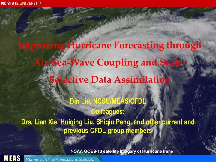
Improving Hurricane Forecasting through Air-Sea-Wave Coupling and Scale-Selective Data Assimilation. Bin Liu, NCSU/MEAS/CFDL Colleagues: Drs. Lian Xie, Huiqing Liu, Shiqiu Peng, and other current and previous CFDL group members. NOAA GOES-13 satellite Imagery of Hurricane Irene.

E N D
Improving Hurricane Forecasting through Air-Sea-Wave Coupling and Scale-Selective Data Assimilation Bin Liu, NCSU/MEAS/CFDL Colleagues: Drs. Lian Xie, Huiqing Liu, Shiqiu Peng, and other current and previous CFDL group members NOAA GOES-13 satellite Imagery of Hurricane Irene
TC forecast error trends for the Atlantic Basin From http://www.nhc.noaa.gov The specific goals of the HFIP are to reduce the average errors of hurricane track and intensity forecasts by 20% within five years (2014) and 50% within 10 years (2019) with a forecast period out to seven days. (From HFIP’s Strategic Plan)
Outline • Air-Sea-Wave Interaction • A Coupled Atmosphere-Wave-Ocean Modeling System (CAWOMS) • Limited-Area Model Nesting/Downscaling • A Scale-Selective Data Assimilation (SSDA) technique
Atmospheric Boundary Layer Oceanic Boundary Layer From CBLAST Project
The CAWOMS Schematic of the coupled atmosphere-wave-ocean modeling system
The Model Coupling Toolkit • The coupling between the model components is carried out by using the Model Coupling Toolkit (MCT, Larson et al., 2005; Jacob et al., 2005) Master begin Model Comp 1 t=t0 Init MCT … t=cpltime … t=tend Finalize MCT Model Comp 2 t=t0 Init MCT … t=cpltime … t=tend Finalize MCT MCT Master end
Atmosphere-ocean coupling • Atmospheric model drives ocean model • WRF drives POM through atmospheric forcing • Oceanic feedback effects • POM provides sea surface temperature to WRF to estimate air-sea heat fluxes • POM provides sea surface currents to determine the relative wind speed for estimation of sea surface wind stress
Wave-ocean coupling • Wave-ocean interaction • Doppler shift effect of background current on waves • Water level variation changing water depth • Modifying upper-ocean currents through radiation stress • Wave-enhanced bottom stress due to wave orbital velocity • Wave-enhanced upper-ocean mixing due to wave breaking • Both wave state and surface ocean conditions impact air-sea momentum and heat fluxes
Atmosphere-wave coupling • Atmospheric model drives wave model • WRF drives SWAN through surface wind • WRF provide surface variables for estimation of sea spray fluxes • Wave-related feedback effects • Wave state and sea spray affected sea surface roughness • Wave state affected sea spray heat fluxes • Dissipative heating
Air-sea momentum flux Wind stress Drag coefficient Sea surface roughness
Sea surface roughness Based on the dependence of sea surface roughness on wind speed, Charnock (1955) proposed the famous Charnock relation E.g., Wu (1980): A constant Charnock parameter corresponds to the drag coefficient increasing linearly with wind speed. Cd-U10 relationships
Wave-age-dependent sea surface roughness • The SCOR workgroup 101 (Jones and Toba 2001) presented a relation between the Charnock parameter and wave age (SCOR relation): • According to this relation, the non-dimensional sea surface roughness first increases and then decreases with the increasing wave age. The SCOR relation and its comparison with various field and laboratory observations (from Toba et al., 2006)
Sea surface under hurricane winds Photo by Mike Black, NOAA/AOML/HRD
Wave state and sea spray affected sea surface roughness Instead of using a constant Charnock parameter, we combined the SCOR relationship (Jones and Toba 2001) with the resistance law of Makin (2005), which took into account of sea sprays impact on air-sea momentum flux, and obtained a sea surface roughness applicable to both low-to-moderate and high wind conditions:
Wave state and sea spray affected sea surface wind stress The wave state and sea spray affected Cd-U10 relationship together with the field and laboratory observations
Wave state and sea spray affected sea surface scalar roughness • As for the sea surface heat and moisture fluxes, we use the parameterization of sea surface scalar roughnesses in COARE algorithm V3.1 (Fairall et al., 2003) to estimate the direct air-sea heat fluxes. The Reynolds number of sea surface aerodynamic roughness
Sea sprays and air-sea heat fluxes Sea spray droplets From Andreas (1995) Droplet Evaporation Layer (DEL) From Andreas and DeCosmo (2002)
Wave state affected sea spray heat flux • By using the wave state dependent Sea Spray Generation Function (SSGF) and Andreas (1992)’s algorithm to estimate nominal sea spray heat flux, and considering the feedback effects • One can now estimate the sea spray sensible and latent heat fluxes that include wave state effect. and are determined following Bao et al. (2000), while is taken as 1 (Andreas, 1992).
Sea state affected air-sea heat fluxes The given atmospheric and sea surface environment: sea surface pressure: 1000 hPa; air temperature: 25 °C; air relative humidity: 80%; neutral stable atmospheric layer; sea surface temperature: 27 °C; and ocean salinity: 34 psu.
CAWOMS - Idealized TC • A bogus vortex with a maximum wind speed of 30 m s-1 at a radius of 70 km is implanted in the ambient atmosphere with uniform easterly winds of 5 m s-1. • The ambient temperature and humidity (salinity) profiles are derived from the monthly averaged vertical profiles for September at the location of (20N, 145E): • NCEP-DOE AMIP-II Reanalysis • One degree WOA05 • The initial SST equals 29 Celsius degree, with a mixed layer depth (MLD) of 40 m. u = -5 m/s Vortex: max wind 30 m/s Typical tropical atmosphere Typical tropical ocean
Experiment design for an idealized TC Summary of the experiments
45-h results of the control run Vertical cross section of potential temperature and horizontal wind speed.
Effects of atmosphere-wave-ocean coupling CTRL CPLAW CTRL CPLAW CTRL CPLAW CPLAO CPLAWO CPLAO CPLAWO CPLAO CPLAWO SWH SSC Wind and SLP
CTRL CPLAW Left: SST Middle: MLD Right: HHC CPLAO CPLAWO
CTRL CPLAW Left: Total upward sensible heat flux Right: Total upward latent heat flux CPLAO CPLAWO
CPLAW CPLAWO HSS HEE HLL HSD CPLAW CPLAWO HLD
Effects of atmosphere-wave-ocean coupling Time series of the simulated (a) minimum SLP, (b) max 10-m wind, (c) maximum SWH, and (d) minimum SST for each experiment. CTRL: Blue CPLAW: Red CPLAO: Green CPLAWO: Black
Sensitivity to MLD *80 => initial MLD of 80 m *120 => initial MLD of 120 m
Summary of AWO interaction and coupling • A CAWOMS consists of WRF, SWAN and POM, based on atmosphere-wave, atmosphere-ocean, and wave-current interaction processes. • The AW coupling has overall positive contribution, which strengthens the TC system. • The AO coupling has overall negative contribution due to the negative feedback of SST cooling, which weakens the TC system. • The overall effects of AWO coupling on TC intensity depend on the balance between wave-related overall positive feedback and oceanic overall negative feedback.
Outline • Air-Sea-Wave Interaction • A Coupled Atmosphere-Wave-Ocean Modeling System (CAWOMS) • Limited-Area Model Nesting/Downscaling • A Scale-Selective Data Assimilation (SSDA) technique
SSDA—A nesting/downscaling technique SSDA L k 10000 km 1000 km 100 km 10 km GCM LAM Sub-grid scale 100 km 12 km Resolution
Traditional sponge zone method and the SSDA approach Domain boundary Relaxation zone Domain interior
The SSDA system and procedure t LAM-WRF Components: LAM (WRF), 3DVAR (WRFDA), Low- and band-pass filter
Application to regional climate simulation of North Atlantic (Jun-Oct 2005) GFS CTRL SSDA The large-scale wind field at 200 hPa for (a) GFS analysis; (b) control run; and (c) SSDA5 at 00 UTC 24 September 2005 (right after the data assimilation cycle).
Application to TC track hindcastingHurricane Katrina (2005) CTRL: Blue SSDA: Red BEST: Black Simulated storm tracks of Hurricane Katrina for experiments (blue ‘o’) CTRL, (green ‘+’) FDDA, and (red ‘x’) SSDA, together with (black ‘s’) the best track
Application to TC track hindcastingHurricane Katrina (2005) CTRL1: Blue ‘o’ SSDA1: Blue ‘*’ CTRL2: Green ‘+’ SSDA2: Green ‘x’ BEST: Black Model domains Simulated storm tracks: (‘o’) CTRL1, (‘*’) SSDA1, (‘+’) CTRL2, (‘x’) SSDA2, together with (‘s’) the best track
Application to TC forecastingHurricane Felix (2007) Track Intensity Mean track (left) and intensity (right) forecast errors for the CTRL and SSDA runs, the GFS global forecasts, the CLIPPER5 or SHF5 model, and the official NHC forecasts, at different forecast periods.
The Hybrid SSDA System LAM-WRF Components: LAM (WRF), 3DVAR (WRFDA), Low- and band-pass filter
Hybrid SSDADA for Hurricane Irene OBS Surface OBS Upper Air
Hybrid SSDADAHRD for Hurricane Irene TDR wind H*Wind
Hybrid SSDA for Hurricane Irene Blue: CTRL Green: SSDA Red: SSDADA Cyan: SSDADAHRD Purple: BEST
Hybrid SSDA for Hurricane Irene CTRL SSDA SSDADA SSDADAHRD Valid at 12Z25AUG
Summary of SSDA • The SSDA approach drives the regional model from the model domain interior in addition to through the conventional sponge zone boundary conditions. • The SSDA approach can be applied in various situations, including regional climate downscaling and tropical cyclone forecasting. The SSDA approach can effectively improve the TC forecasting by assimilating large-scale information from global model results, especially for the track forecasting. • The Hybrid SSDA approach has an additional function (merit) to assimilate all kinds of available observations, leading to improvements for both TC intensity and track forecasting.
A Hybrid SSDA-CAWOMS TC Intensity Forecasting TC Track Forecasting CAWOMS SSDA DA Hybrid SSDA Hybrid SSDA-CAWOMS TC Track and Intensity Forecasting