Download
1 / 33
330 likes | 345 Views
Nearest Neighbor Search in high-dimensional spaces. Alexandr Andoni (Princeton/CCI → MSR SVC) Barriers II August 30, 2010. Nearest Neighbor Search (NNS). Preprocess: a set D of points in R d Query: given a new point q , report a point p D with the smallest distance to q. p. q.

E N D
Nearest Neighbor Searchin high-dimensional spaces Alexandr Andoni (Princeton/CCI → MSR SVC) Barriers II August 30, 2010
Nearest Neighbor Search (NNS) • Preprocess: a set D of points in Rd • Query: given a new point q, report a point pDwith the smallest distance to q p q
Motivation • Generic setup: • Points model objects (e.g. images) • Distance models (dis)similarity measure • Application areas: • machine learning, data mining, speech recognition, image/video/music clustering, bioinformatics, etc… • Distance can be: • Euclidean, Hamming, ℓ∞, edit distance, Ulam, Earth-mover distance, etc… • Primitive for other problems: • find the closest pair in a set D, MST, clustering… p q
Plan for today 1. NNS for basic distances 2. NNS for advanced distances: embeddings 3. NNS via product spaces
2D case • Compute Voronoi diagram • Given query q, perform point location • Performance: • Space: O(n) • Query time: O(log n)
High-dimensional case • All exact algorithms degrade rapidly with the dimension d • When d is high, state-of-the-art is unsatisfactory: • Even in practice, query time tends to be linear in n
Approximate NNS c-approximate • r-near neighbor: given a new point q, report a point pDs.t.||p-q||≤r cr r as long as there exists a point at distance ≤r p cr q
Approximation Algorithms for NNS • A vast literature: • With exp(d) space or Ω(n) time: [Arya-Mount-et al], [Kleinberg’97], [Har-Peled’02],… • With poly(n) space and o(n) time: [Kushilevitz-Ostrovsky-Rabani’98], [Indyk-Motwani’98], [Indyk’98, ‘01], [Gionis-Indyk-Motwani’99], [Charikar’02], [Datar-Immorlica-Indyk-Mirrokni’04], [Chakrabarti-Regev’04], [Panigrahy’06], [Ailon-Chazelle’06], [A-Indyk’06]…
The landscape: algorithms Space: poly(n). Query: logarithmic Space: small poly (close to linear). Query: poly (sublinear). Space: near-linear. Query: poly (sublinear).
Locality-Sensitive Hashing [Indyk-Motwani’98] q • Random hash function g: RdZ s.t. for any points p,q: • If ||p-q|| ≤ r, then Pr[g(p)=g(q)] is “high” • If ||p-q|| >cr, then Pr[g(p)=g(q)] is “small” • Use several hash tables p • “not-so-small” Pr[g(p)=g(q)] :nρ, whereρs.t. 1 P1 P2 ||p-q|| r cr
Example of hash functions: grids [Datar-Immorlica-Indyk-Mirrokni’04] • Pick a regular grid: • Shift and rotate randomly • Hash function: • g(p) = index of the cell of p • Givesρ≈ 1/c p
State-of-the-art LSH [A-Indyk’06] p • Regular grid → grid of balls • p can hit empty space, so take more such grids until p is in a ball • Need (too) many grids of balls • Start by reducing dimension to t • Analysis gives • Choice of reduced dimension t? • Tradeoff between • # hash tables, n, and • Time to hash, tO(t) • Total query time: dn1/c2+o(1) p 2D Rt
q P(r) x p Proof idea • Claim: , where • P(r)=probability of collision when ||p-q||=r • Intuitive proof: • Let’s ignore effects of reducing dimension • P(r) = intersection / union • P(r)≈random point u beyond the dashed line • The x-coordinate of u has a nearly Gaussian distribution → P(r) exp(-A·r2) r q p u
The landscape: lower bounds Space: poly(n). Query: logarithmic Space: small poly (close to linear). Query: poly (sublinear). Space: near-linear. Query: poly (sublinear).
Challenge 1: • Design space partitioning of Rt that is • efficient: point location in poly(t) time • qualitative: regions are “sphere-like” c2 [Prob. needle of length 1 is cut] ≥ [Prob needle of length c is cut]
NNS for ℓ∞ distance [Indyk’98] • Thm: for ρ>0, NNS for ℓ∞d with • O(d * log n) query time • n1+ρ space • O(lg1+ρ lg d) approximation • The approach: • A deterministic decision tree • Similar to kd-trees • Each node of DT is “qi < t” • One difference: algorithms goes down the tree once (while tracking the list of possible neighbors) • [ACP’08]: optimal for decision trees! q1<5 ? Yes No q2<4 ? q2<3 ? Yes No q1<3 ?
Plan for today 1. NNS for basic distances 2. NNS for advanced distances: embeddings 3. NNS via product spaces
What do we have? • Classical ℓp distances: • Hamming, Euclidean, ℓ∞ How about other distances, like edit distance? ed(x,y) = number of substitutions/insertions/ deletions to transform string x into y Hamming (ℓ1) Euclidean (ℓ2) ℓ∞
NNS via Embeddings • An embeddingof M into a host metric (H,dH)is a map f : M→H • has distortionA ≥ 1if x,y M dM(x,y) ≤ dH(f(x),f(y)) ≤ A*dM(x,y) • Why? • If H is Euclidean space, then obtain NNS for the original space M ! • Popular host: H = ℓ1 f f
Embeddings of various metrics • Embeddings into ℓ1 Challenge 2: Improve the distortion of embedding edit distance into ℓ1
A barrier: ℓ1non-embeddability • Embeddings into ℓ1
Other good host spaces? • What is “good”: • is algorithmically tractable • is rich (can embed into it) , etc (ℓ2)2=real space with distance: ||x-y||22 (ℓ2)2, host with v. good LSH (sketching l.b. via communication complexity) ̃ [AK’07] [AK’07] [AIK’08]
Plan for today 1. NNS for basic distances 2. NNS for advanced distances: embeddings 3. NNS via product spaces
d1 d1 … … d∞,1 d∞,1 α Meet a new host d1 … β Iterated product space, Ρ22,∞,1= d∞,1 d22,∞,1 γ
Why Ρ22,∞,1 ? [A-Indyk-Krauthgamer’09, Indyk’02] edit distance between permutations • Because we can… • Embedding: …embed Ulam into Ρ22,∞,1 with constant distortion • (small dimensions) • NNS: Any t-iterated product space has NNS on n points with • (lg lg n)O(t) approximation • near-linear space and sublinear time • Corollary: NNS for Ulam with O(lg lg n)2 approximation • cf. each ℓp part has logarithmic lower bound!
Embedding into • Theorem: Can embed Ulam metric into Ρ22,∞,1 with constant distortion • Dimensions:α=β=γ=d • Proof intuition • Characterize Ulam distance “nicely”: • “Ulam distance between x and y equals the number of characters that satisfy a simple property” • “Geometrize” this characterization
Ulam: a characterization E.g., a=5; K=4 X[5;4] • Lemma: Ulam(x,y) approximately equals the number characters a satisfying: • there exists K≥1 (prefix-length) s.t. • the set of K characters preceding a in xdiffers muchfrom the set of K characters preceding a in y 123456789 x= y= 123467895 Y[5;4]
Ulam: the embedding X[5;4] 123456789 • “Geometrizing” characterization: • Gives an embedding 123467895 Y[5;4]
A view on product metrics: • Give more computational view of embeddings • Ulam characterization is related to work in the context of property testing & streaming [EKKRV98, ACCL04, GJKK07, GG07, EJ08] sum of squares (ℓ22) edit(P,Q) max (ℓ∞) sum (ℓ1) P Q
Challenges 3,… • Embedding into product spaces? • Of edit distance, EMD… • NNS for any norm (Banach space) ? • Would help for EMD (a norm) • A first target: Schatten norms (e.g., trace of a matrix) • Other uses of embeddings into product spaces? • Related work: sketching of product spaces [JW’09, AIK’08, AKO]
Some aspects I didn’t mention yet • NNS for spaces with low intrinsic dimension: • [Clarkson’99], [Karger-Ruhl’02], [Hildrum-Kubiatowicz-Ma-Rao’04], [Krauthgamer-Lee’04,’05], [Indyk-Naor’07],… • Cell-probe lower bounds for deterministic and/or exact NNS: • [Borodin-Ostrovsky-Rabani’99], [Barkol-Rabani’00], [Jayram-Khot-Kumar-Rabani’03], [Liu’04], [Chakrabarti-Chazelle-Gum-Lvov’04], [Pătraşcu-Thorup’06],… • NNS for average case: • [Alt-Heinrich-Litan’01], [Dubiner’08],… • Other problems via reductions from NNS: • [Eppstein’92], [Indyk’00],… • Many others !
Summary of challenges • 1. Design qualitative, efficient space partitioning • 2. Embeddings with improved distortion: edit into ℓ1 • 3. NNS for any norm: e.g. trace norm? • 4. Embedding into product spaces: say, of EMD