Download
1 / 51
510 likes | 967 Views
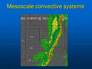
Mesoscale convective systems. Presented by Wes Junker At COMET For the Hydrometeorology Faculty Course 2000 Monday, 12 June 2000. Mesoscale convective systems. Come in a variety of sizes and shapes

E N D
Mesoscale convective systems Presented by Wes Junker At COMET For the Hydrometeorology Faculty Course 2000 Monday, 12 June 2000
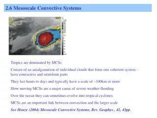
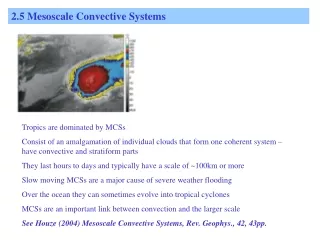
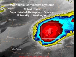
Mesoscale convective systems • Come in a variety of sizes and shapes • MCSs account for 30-70 percent of precipitation during the warm season (Apr-Sept.) (Fritsch et al, 1986* , • Kane et al., (1987*) Found precipitation characteristics of MCS are similar to those of MCCs except for size. • Larger MCCs tend to produce more cumulative rainfall and to a lesser extent point rainfall. (McAnelly and Cotton, 1989 MWR). • Smaller MCSs typically are of shorter duration (Geerts, WAF 1998) • Large MCCs in Plains generally reach their peak size and intensity at about midnight (Houze MWR 1990). • However, between 35N and 35S, MCSs are twice as likely at sunset than sunrise (Mohr and Zipser, BAM 1996). *J. Climate Appl. Meteor., 1986)
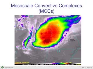
Maddox et al. MCC papers revolutionized summer forecasting of precipitation. The paper noted the ingredients a forecaster should look for when anticipating an MCC that might produce a flash flood. • MOST ARE ASSOCIATED WITH MCCs OR MCSs AND OCCUR AT NIGHT • ABNORMALLY MOIST, PWS USUALLY ARE 1.40” OR HIGHER AND AVERAGE ABOUT 1.62”. • VERTICAL SHEAR IS WEAK TO MODERATE ALLOWING SLOW MOVEMENT • MANY OCCUR NEAR THE 500 MB RIDGE POSITION • OCCUR AT THE NOSE OF THE LOW LEVEL WIND MAXIMUM FROM MADDOX ET AL., 1979
FRONTAL AND MESOHIGH (850 MB)Why does the orientation of the low-level jet favor heavy rainfall? (From Maddox et al. 1980) Td=14 oC Max Winds Td=10 oC Td=12 oC Max Winds Axis of Td=14 oC Axis of 120 nm 120 nm MESOHIGH Td=16 oC FRONTAL SCALE IS USUALLY SMALLER FOR MESOHIGH EVENTS (Kane et al., 1987, J. Climate Appl. Meteor., 26, 1345-1357)
SURFACE MESOHIGH OUTFLOW BOUNDARY BUBBLE HIGH COOL AND MOIST H L WARM AND MOIST Td=70oF Td=60oF Td=70oF 120 nm Td=60oF Mesohigh or Frontal TypeOutflow boundary or front provides focus for lifting. The area at highest risk for heavy rainfall is in red. H SURFACE FRONTAL Td=60oF COOL AND MOIST L WARM AND MOIST H Td=70oF Td=70oF Td=60oF 120 nm
-57 200 MB MESOHIGH -36 300 10 PW=1.64” -10 500 (162%) 6 7 700 4 K=39 18 850 SI=-5 3 1014 71 SFC 66 -56 200 MB -36 300 FRONTAL 15 -10 PW=1.60” 6 500 (158%) 7 700 3 K=38 17 850 SI=-4 4 1013 SFC 70 65
About 60% of mesohigh and frontal type heavy rainfall events occur near the ridge axis. 500 mb 500 mb MOIST MOIST H FRONTAL MESOHIGH 120 nm Maddox et al., 1980
NEAR RIDGE AXIS YOU HAVE EITHER WEAK INERTIAL STABILITY OR INERTIAL INSTABILITY. AREAS WITH STRONG ANTICYCLONIC SHEAR HAVE WEAK INERTIAL STABILITY OR INERTIAL INSTABILITY
Two Conceptual diagrams of the structure of an warm core MCS, from a circulation perspective on left (Scofield and Junker 1988), and from an PV anomaly perspective on right (Fritsch et al., JAS, 1994)
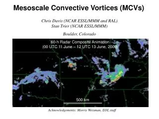
Mesoscale convective vortices • Convection redevelops on afternoon and then strengthens during night. • During day convection tends to develop on periphery near outflow boundary, at night often redevelops near center of vortex. (Bartels and Maddox, MWR 1991) 0300 UTC 0330 UTC Figure from Fritsch et al, (JAS, 1994) 0900 UTC 0500 UTC
Latitudinal and monthly distribution of MCC centroids at maximum extent. Contours represent average distribution for period 1978-1985. Dots make up individual yearly distribution, a) for 1986, b) 1987. Shaded area indicates null period From Augustine and Howard (MWR,1991)
850 analysis of heights, temps, winds (full barb 5 ms-1. Dark and light shaded areas depict the 12 and 10 g kg-1 mean mixing ratio. On left null period, on right active period. From Augustine and Howard (MWR,1991) MCCs need mositure and instability to form.
MCS area at maximum extent versus maximum 850 mb frontogenesis in the vicinity of the location of the maximum extent at 00 UTC. L=large MCC, Small MCS From Augustine and Caracena , 1994, Wea. Forecasting
Normalized composite precipitation (mm) pattern for 74 MCCs. Dashed and dotted lines are approximate centroid tracks of -32 and -54oC cloud-shields, respectively. The horizontal axis is the axis of propagation and indicates the storm heading Cluster around propagation axis the probability of 1 mm of rain is 100% but for 75 mm drops to 10% nearly coincident with the 35 mm shown in figure above. From Kane et al., 1987*
MCSs can develop a number of ways. Mature systems have a convective and “stratiform” precipitation shield Stratiform rainfall can produce up to 50% of rain in some MCSs Loerer and Johnson, Wea. Forecasting 1995
Predictions of MCS symmetry and movement play a significant role in determining precipitation amounts Possible cause of asymmetry 1) The Coriolis force acting upon the ascending front-to-rear flow turns the flow to the north, leading to an accumulation of hydrometeors and buoyancy Loerer and Johnson, Wea. Forecasting 1995 2) The Coriolis force acting on the surface cold pool helps drive cold air south leading to new cell generation 3). Position of low-level jet and strongest instability.
How does stratiform precipitation form • From front to rear ascending air creating anvil • melting of ice or snow crystals which induce cool pool just below freezing level • this tightens thermal gradient and is frontogenetic. • Thermally direct circulation enhances lifting above freezing level and subsidence below it. From Szeto et al, 1988 JAS
MCSs over Southeast • Are about twice as common is summer as winter • occur mostly in afternoon but the amplitude of occurrence in the afternoon is not as great as for general thunderstorms • despite being more common in summer, the probability of any point being affected by an MCS is about the same for winter as summer • in summer-usually are small and short lived • in winter-are larger and longer lived • in winter do not evolve into typical leading line trailing stratiform precipitation very often.
35 360 30 330 25 300 20 Observed cell speed during MCC genesis 270 Observed cell direction during MCC genesis 15 240 10 5 r=.71 r=.76 210 0 180 360 0 210 270 300 240 330 5 25 10 180 15 20 30 35 Mean 850-300 mb wind speed Mean 850-300 mb wind direction Individual cells move approximately with the 850-300 mean wind during early stages of an MCS From Corfidi et al, 1996
300 240 180 120 60 r=.65 180 420 480 300 360 240 Direction of MBE propagation The direction of the MBE (the most active part of the MCS) is dependent on the direction of the low-level jet (Corfidi et al., 1997) and on the position of the most moist and unstable air relative to the MCS. The direction of propagation is in the opposite direction of the low-level jet. This may be why MCCs tend to track to the right of the mean wind. Direction of low-level jet Systems with propagation vectors between 0-120 degrees have been plotted between 360 and 480 degrees From Corfidi
Movement of convective systems • Individual cells movement can be approximated using the mean wind • Movement of an MCS is dependent on, 1) the mean flow between 850-300 mb (Corfidi, 1994), and 2) the rate new cells are growing (propagation) • The propagation rate is strongly dependent on the low-level jet but is also dependent on the strength of the cold pool • The stronger the low-level jet (compared to the mean wind), the more the MCS will deviate from the mean wind.
1. FORWARD DIRECTION OF PROPAGATION MCS AXIS OF LOW-LEVEL JET UNSTABLE AIR 1000-500 THICKNESS 2. BACKWARD N E W ADOPTED FROM JIANG AND SCOFIELD, 1987 S UNSTABLE AIR THE PROPAGATION OF A CONVECTIVE SYSTEM IS DEPENDENT ON THE LOCATION OF: 1) THE MOST UNSTABLE AIR, 2) THE AXIS AND ORIENTATION OF THE LOW-LEVEL JET, AND 3) THE LOCATION OF THE STRONGEST LOW-LEVEL MOISTURE CONVERGENCE
Area with most unstable Lifted Indices shaded. 35 TO 40 kt winds are feeding across KS into NE An almost e-w frontal band with PWS 1.80” or higher (shaded) An example of a quasi-stationary convective system The most unstable air is usually found upstream of the initial convection during backbuilding or quasi-stationary convective events JUNKER AND SCNEIDER, 1997, NAT. WEA. DIGEST, ,21, 5-17
Factors favorable to quasi-stationary convection 1)mean winds almost parallel to the front but directed slightlyaway from it 2) a low-level 1e ridge to west, and 3) the location of the strongest moisture convergence west of the initial convection 00Z 00Z 1000-850 mb layer mean moisture flux (vectors)moisture flux magnitude (dashed) and moisture flux divergence (-4 x10⁻⁷s-1 are shaded), the red dot represents the location where convection started 850-300 mb mean winds, 982 mb equivalent potential temperature (dashed) and msl pressure (solid) JUNKER AND SCNEIDER, 1997, NAT. WEA. DIGEST, ,21, 5-17
MOISTURE CONVERGENCE STRENGTHENS OVER EASTERN NE AS PRESSURES FALL IN RESPONSE TO THE APPROACH OF A WEAK SURFACE WAVE 21Z 00Z 03Z 06Z MSL PRESSURE (THICK SOLID), MOISTURE CONVERGENCE (HIGHEST VALUES SHADED), RED DOT IS WHERE INITIAL CELL FORMED THE WIND AND MOISTURE CONVERGENCE FIELDS CAN CHANGE RAPIDLY AS A RESULT OF PRESSURE RISES OR FALLS.
1st cell 00Z 21Z New cells form upstream Merger Accumulated precipitation from the storm 02Z 06Z DURING THE 1993 DSM FLASH FLOOD, THE CONVECTIVE SYSTEM REMAINED STATIONARY FOR ABOUT 9 HOURS, WHY?
Investigation of the MCS during the Great Flood of 1993 • MCSs were investigated for June-Sept. • all 2, 3, 4 and 5 inch areas were measured for each MCS identified • systems were categorized based on the size of the 3” coverage • The largest scale, heaviest events were compared with smaller scale events that produced less rain.
Average size of various precipitation thresholds for each category (km2)during June-Sept. 1993, (Junker et al 1999 WAF)
Cases where lower relative humidity and/or a stronger cap are more likely to have the convection form north of the front. 552 558 L 564 THICKNESS VALUES FOR 70% SATURATION PW=0.80” P.W. THICKNESS P.W. THICKNESS INFLOW 570 522 561 .22 .90 528 564 .27 1.05 =CONVECTIVE AREA 534 567 .35 1.15 552 540 1.25 570 .43 558 L 564 573 .55 1.40 546 outflow boundary 552 .70 576 1.55 PW=1.15” .80 558 579 1.70 561 .90 570 582 1.90 INFLOW From Funk (WAF, 1991)
THE LARGER SCALE HEAVY RAINS FELL WITH HIGHER RH VALUES. THERE WERE CATEGORIES BASED ON THE AREAL EXTENT OF THE 4 INCH. CAT 1 HAS NO 3 INCH AREA, WHILE CAT 4 HAD 3600 SQ. NAUTICAL MI. OR MORE Junker et al 1999 WAF The fact that few larger scale heavy rainfall events occurred to the of the line may be the reason preferred thickness appears to work
The maximum observed rainfall at a point versus the size of the 2” area Junker et al 1999 WAF
When the moisture convergence is aligned with the 850-300 mb mean flow, a sizeable area of 3” precipitation is more likely. THE Y-AXIS REPRESENTS THE LENGTH OF THE -2X10⁻⁷ S-1 OR GREATER MOISTURE FLUX CONVERGENCE MEASURED UPSTREAM ALONG A LINE DEFINED BY THE MEAN FLOW. a 3” area is 3600 sq. nm less likely area of 3” more likely (inches) Junker et al 1999 WAF
LARGEST 3” CAT 4 AVERAGE SIZE OF THE 3” FOR THE VARIOUS CATEGORIES, NOTE THE SMALL SCALE OF THE MOST INTENSE RAINFALL. THE BOTTOM RIGHT FIGURE IS THE LARGEST 3” DURING THE STUDY CAT 3 CAT 1 CAT 2 BECAUSE OF THE SMALL SCALE, IT IS VERY HARD TO CORRECTLY FORECAST THE CORE OF HEAVIEST RAINS. SOME KIND OF PROBABILISTIC APPROACH TO FORECASTING MAY BE BETTER THAN A DETERMINISTIC ONE
ALL THE CATEGORY EVENTS OCCURRED WITH PWS AT OR ABOVE 1.40”. IN GENERAL THE SHEAR WAS WEAK TO MODERATE (Mean winds are in knots) Junker et al 1999 WAF
700 mb temperatures above 12oC appear to limit the size of any convective system that forms. The HPC rule of thumb that 700 mb temperatures above 12oC will provide an effective cap is a decent first guess BUT you should also look at the negative area on the sounding
COMPOSITE OF 12 LARGEST EVENTS, THE HEAVIEST RAIN OCCURS AT THE NOSE OF THE LOW-LEVEL JET IN/OR NEAR THE STRONGEST WARM ADVECTION • 850 MB WIND DIRECTION (ARROWS) AND ISOTACHS ON LEFT, 850 MB TEMPERATURE ADVECTION ON RIGHT, BLACK DOT IS CENTER OF HEAVIEST RAIN, 2 BY 2 DEG. LATITUDE GRID 1
The moisture transport (flux or qV) and moisture convergence are dependent on the low-level jet. 8 6 • 850 mb moisture flux (left) and moisture flux divergence (right). Note that the heaviest rain occurred southeast of the strongest 850 mb moisture convergence. The red dot is the center of heaviest rainfall. 7 4 6 8 2 10 0 17 -2 9 19 18 -4 -6 -8 0 -4 -6 -2 2 4 -8 6 8
THE HEAVIEST RAIN USUALLY OCCURS TO THE NORTHEAST OF THE THETA-E RIDGE, NEAR BUT JUST SOUTH OF THE MAXIMUM IN THETA-E ADVECTION THETA-E (1e) VCL1e
IN SUMMARY • The scale of precipitation associated with an MCS during the study appears to be related to • the relative humidity • the orientation of the moisture convergence band with respect to the mean flow • the width of the axis of stronger moisture convergence
In summary (continued) • Most of the MCSs formed to the north or northeast of the strongest 850 mb winds and moisture flux. • Most occurred in an area of 850 mb warm and theta-e advection • most occurred on the southern edge of the 250 mb divergence • the size of the heavy rainfall seems to be modulated at least in part by the RH and by the orientation of the moisture convergence to the mean flow
LOCATION OF COMPOSITE CASES 2 4 4 4 1 1 4 1 4 2 4 4 2 1 1 2 2 1 1 2 3 1 3 3 2 2 1 2 3 1 3 2 2 1 2 2 2 1 1 1 2 2 1 LEGEND 2 SYNOPTIC TYPE #EVENTS (45) 1 BLOCKING ANTICYCLONE 15 2 DEFORMATION ZONE 17 3 SHORTWAVE TROUGH IN NORTHWEST FLOW 6 SHORTWAVE TROUGH IN ZONAL FLOW 4 7 MCCs IN WEST, CLIMATOLOGYLOCATIONS OF LARGEST 45 MCS/MCC SYSTEMS USED TO PREPARE 4 TYPES OF ATMOSPHERIC COMPOSITES Scale is usually smaller than East, so small, that predicting where the MCS will occur is almost impossible. PWs OF 1.00” ARE HIGH 700 MB (DEWPOINTS IN WEST ARE TYPICALLY IN THE 6-8oC RANGE WHEN SIGNFICANT FLASH FLOODS OCCUR) SURFACE DEWPOINTS ARE IN THE 50S FROM CHAPPELL COMET NOTES
SOME CLIMATOLOGYFREQUENCY OF FLASH FLOODING OR 2”/24HR RAINFALL FOR 137 EVENTS IN WESTNOTE THE HIGH FREQUENCY IN LATE JULY AND AUGUST FROM CHAPPELL COMET NOTES
EVENTS IN INTERMOUNTAIN REGION ALSO HAVE A DISTINCT MAXIMUM DURING THE 6-HR PERIOD BETWEEN 2 PM AND 8 PM LOCAL DAYLIGHT TIME. OCCUR MOSTLY IN AUGUST AND SEPTEMBER INTO EARLY OCTOBER.
The vast majority of front range events occur during the late July and early August, and occur during the late afternoon and early evening hours (2-8 PM) FROM CHAPPELL COMET NOTES
HEAVY RAIN EVENTS ALONG THE FRONT RANGEBIG THOMPSON, FORT COLLINS, CHEYENNE, MADISON COUNTY (VA) • A SLOW MOVING FRONT IS LOCATED UP JUST SOUTH OF THE AREA • WINDS ALOFT ARE LIGHT AND SOUTHEASTERLY • A LARGE AMPLITUDE NEGATIVE-TILTED UPPER RIDGE AXIS LIES NORTH AND EAST OF THE AREA • A WEAK SHORTWAVE ROTATES NORTHWARD TOWARDS THE AREA RESULTING IN WEAK PVA FROM MADDOX ET AL., 1977
H L L L IDEALIZED SURFACE PATTERN Cells develop east of highest terrain* Cells then move slowly north and northwest* Redevelopment occurs on SE or S flank* Heaviest rain falls over a very small area* This pattern also occurs in east (ie. Madison County flash flood. Scale of rain is heaviest rain is small LOW LEVEL JET AND MOISTURE TONGUE THREAT AREA 500 MB TROF Td$65oF LOW LEVEL T-Td#6oC THERMAL AXIS ADOPTED FROM MADDOX ET AL., 1977
ETA 500MB FORECASTSNOTE THE TILT OF THE UPPER RIDGE AXIS. NEGATIVE TILTING RIDGE AXIS L 24 HR V.T. 12Z 12 HR V.T. 00Z
OBSERVED MAPS VALID 00Z .. 7158 169 78 7 61 207 71 6848 71 171 64 51 62 179 205 74 77 5 55 20 65 13 60 7254 173 193 82 193 73 173 68 13 67 64 190 82 63 193 185 76 54 72 Td$15oC 70 8270 66 13 63 0 50 T-Td#6oC . 169 . 72 8365 178 5 63 6556 BOUNDARY? 16 8270 6446 8263 148 131 8566 500 MB SURFACE 850 MB FROM THESE MAPS WHAT CAN BE INFERRED ABOUT THE PRECIPITATION EFFICIENCY OF ANY CELLS THAT FORM?
MODEL 12-36 HR QPF REMEMBER YOU NEED TO KNOW MODEL BAISES $ NGM AVN ETA $.01” WHICH MODEL DO YOU THINK HAS THE BEST FORECAST OF THE SCALE OF THE 2.00” OR GREATER AMOUNTS? WHAT ABOUT THE LOCATION OF THE MAXIMUM RAINFALL? $.50” $1.0” $.2.0” $.3.0”
VERIFICATION 8-10” OF RAIN ON FORT COLLINS & NEARBY FOOTHILLS 4 MILES AWAY ONLY .83” OBSERVED $.50” 295 HOUSES OR MOBILE HOMES DESTROYED, 4 KILLED $1.0” $2.0” . $3.0” A LARGER MCS MOVED SOUTHEASTWARD AWAY FROM A SMALLER SCALE QUASI-STATIONARY CONVECTIVE STORM. Note the barren dry expanse known as southeast Wyoming VERIFYING ANALYSIS VALID 12Z JULY 29