0 0 0 0 1

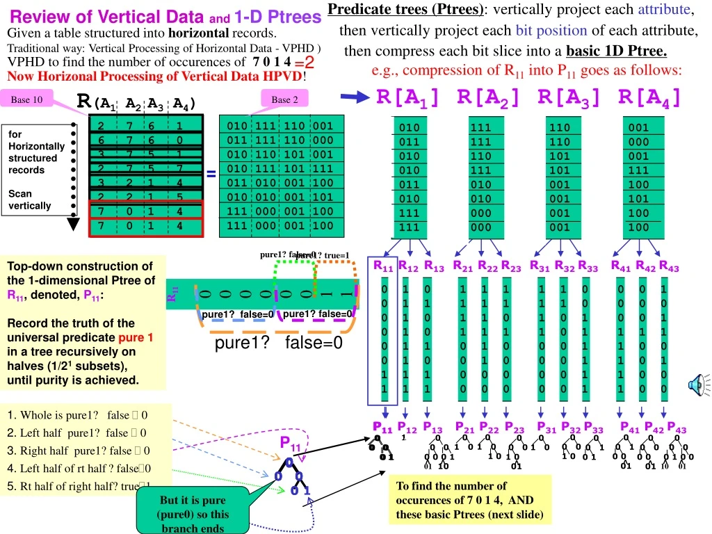
1. Predicate trees (Ptrees): vertically project each attribute, R[A1] R[A2] R[A3] R[A4] 010 111 110 001 011 111 110 000 010 110 101 001 010 111 101 111 011 010 001 100 010 010 001 101 111 000 001 100 111 000 001 100 010 111 110 001 011 111 110 000 010 110 101 001 010 111 101 111 011 010 001 100 010 010 001 101 111 000 001 100 111 000 001 100 for Horizontally structured records Scan vertically = pure1? true=1 pure1? false=0 R11 R12 R13 R21 R22 R23 R31 R32 R33 R41 R42 R43 0 1 0 1 1 1 1 1 0 0 0 1 0 1 1 1 1 1 1 1 0 0 0 0 0 1 0 1 1 0 1 0 1 0 0 1 0 1 0 1 1 1 1 0 1 1 1 1 0 1 1 0 1 0 0 0 1 1 0 0 0 1 0 0 1 0 0 0 1 1 0 1 1 1 1 0 0 0 0 0 1 1 0 0 1 1 1 0 0 0 0 0 1 1 0 0 pure1? false=0 pure1? false=0 pure1? false=0 0 0 0 1 0 01 0 1 0 1 0 1 1. Whole is pure1? false  0 P11 P12 P13 P21 P22 P23 P31 P32 P33 P41 P42 P43 2. Left half pure1? false  0 P11 0 0 0 0 0 01 3. Right half pure1? false  0 0 0 0 0 1 0 0 10 01 0 0 0 1 0 0 0 0 0 0 0 1 01 10 0 0 0 0 1 0 0 0 0 1 0 0 0 0 1 0 0 0 0 0 0 0 0 0 0 1 0 0 ^ ^ ^ ^ ^ ^ ^ 0 0 1 0 1 4. Left half of rt half? false0 0 0 1 0 0 01 5. Rt half of right half? true1 0 1 0 Review of Vertical Data and 1-D Ptrees then vertically project each bit position of each attribute, Given a table structured into horizontal records. Traditional way: Vertical Processing of Horizontal Data - VPHD ) then compress each bit slice into a basic 1D Ptree. e.g., compression of R11 into P11 goes as follows: =2 VPHD to find the number of occurences of 7 0 1 4 Now Horizonal Processing of Vertical Data HPVD! R(A1 A2 A3 A4) Base 10 Base 2 2 7 6 1 6 7 6 0 3 7 5 1 2 7 5 7 3 2 1 4 2 2 1 5 7 0 1 4 7 0 1 4 R11 0 0 0 0 0 0 1 1 Top-down construction of the 1-dimensional Ptree of R11, denoted, P11: Record the truth of the universal predicate pure 1 in a tree recursively on halves (1/21 subsets), until purity is achieved. P11 To find the number of occurences of 7 0 1 4, AND these basic Ptrees (next slide) But it is pure (pure0) so this branch ends

2. R[A1] R[A2] R[A3] R[A4] 010 111 110 001 011 111 110 000 010 110 101 001 010 111 101 111 101 010 001 100 010 010 001 101 111 000 001 100 111 000 001 100 010 111 110 001 011 111 110 000 010 110 101 001 010 111 101 111 101 010 001 100 010 010 001 101 111 000 001 100 111 000 001 100 = R11 R12 R13 R21 R22 R23 R31 R32 R33 R41 R42 R43 0 1 0 1 1 1 1 1 0 0 0 1 0 1 1 1 1 1 1 1 0 0 0 0 0 1 0 1 1 0 1 0 1 0 0 1 0 1 0 1 1 1 1 0 1 1 1 1 1 0 1 0 1 0 0 0 1 1 0 0 0 1 0 0 1 0 0 0 1 1 0 1 1 1 1 0 0 0 0 0 1 1 0 0 1 1 1 0 0 0 0 0 1 1 0 0 0 1 0 1 0 0 0 0 1 0 01 0 1 0 0 1 01 This 0 makes entire left branch 0 7 0 1 4 These 0s make this node 0 P11 P12 P13 P21 P22 P23 P31 P32 P33 P41 P42 P43 These 1s and these 0s(which when complemented are 1's)make this node1 0 0 0 0 0 01 0 0 0 0 1 0 0 10 01 0 0 0 1 0 0 0 0 0 0 0 1 01 10 0 0 0 0 1 10 0 1 0 ^ ^ ^ ^ ^ ^ ^ ^ ^ 0 0 1 0 1 0 0 1 0 0 01 0 1 0 R(A1 A2 A3 A4) 2 7 6 1 3 7 6 0 2 7 5 1 2 7 5 7 5 2 1 4 2 2 1 5 7 0 1 4 7 0 1 4 # change Vertical Data: 1Shortcuts in the processing of 1-Dimensional Ptrees To count occurrences of 7,0,1,4 use 111000001100: 0 P11^P12^P13^P’21^P’22^P’23^P’31^P’32^P33^P41^P’42^P’43 = 0 0 01 The 21-level (2nd level has the only 1-bit so the 1-count of the Ptree is 1*21 = 2 ^

3. F3 = L3 C1 F1 = L1 C2 F2 = L2 C3 C2 Data_Lecture_4.1_ARM itemset Scan D {2 3 5} {1 2 3} {1,3,5} Scan D Scan D P1 2 //\\ 1010 P2 3 //\\ 0111 P1^P2^P3 1 //\\ 0010 Build Ptrees: Scan D P1^P2 1 //\\ 0010 P3 3 //\\ 1110 P1^P3 ^P5 1 //\\ 0010 P1^P3 2 //\\ 1010 P4 1 //\\ 1000 P2^P3 ^P5 2 //\\ 0110 P5 3 //\\ 0111 P1^P5 1 //\\ 0010 L2={13}{23}{25}{35} L1={1}{2}{3}{5} L3={235} P2^P3 2 //\\ 0110 P2^P5 3 //\\ 0111 P3^P5 2 //\\ 0110 HTT {123} pruned since {12} not frequent {135} pruned since {15} not frequent Example ARM using uncompressed Ptrees(note: I have placed the 1-count at the root of each Ptree)

4. L3 L1 L2 Data_Lecture_4.1_ARM 1-ItemSets don’t support Association Rules (They will have no antecedent or no consequent). 2-Itemsets do support ARs. Are there any Strong Rules supported by Frequent=Large 2-ItemSets(at minconf=.75)? {1,3} conf({1}{3}) = supp{1,3}/supp{1} = 2/2 = 1 ≥ .75 STRONG conf({3}{1}) = supp{1,3}/supp{3} = 2/3 = .67 < .75 {2,3} conf({2}{3}) = supp{2,3}/supp{2} = 2/3 = .67 < .75 conf({3}{2}) = supp{2,3}/supp{3} = 2/3 = .67 < .75 {2,5} conf({2}{5}) = supp{2,5}/supp{2} = 3/3 = 1 ≥ .75STRONG! conf({5}{2}) = supp{2,5}/supp{5} = 3/3 = 1 ≥ .75STRONG! {3,5} conf({3}{5}) = supp{3,5}/supp{3} = 2/3 = .67 < .75 conf({5}{3}) = supp{3,5}/supp{5} = 2/3 = .67 < .75 Are there any Strong Rules supported by Frequent or Large 3-ItemSets? {2,3,5} conf({2,3}{5}) = supp{2,3,5}/supp{2,3} = 2/2 = 1 ≥ .75STRONG! conf({2,5}{3}) = supp{2,3,5}/supp{2,5} = 2/3 = .67 < .75 No subset antecedent can yield a strong rule either (i.e., no need to check conf({2}{3,5}) or conf({5}{2,3}) since both denominators will be at least as large and therefore, both confidences will be at least as low. conf({3,5}{2}) = supp{2,3,5}/supp{3,5} = 2/3 = .67 < .75 No need to check conf({3}{2,5}) or conf({5}{2,3}) DONE!

5. Ptree-ARM versus Apriori on aerial photo (RGB) data together with yeild data P-ARM compared to Horizontal Apriori (classical) and FP-growth (an improvement of it). • In P-ARM, we find all frequent itemsets, not just those containing Yield (for fairness) • Aerial TIFF images (R,G,B) with synchronized yield (Y). Scalability with number of transactions Scalability with support threshold • Identical results • P-ARM is more scalable for lower support thresholds. • P-ARM algorithm is more scalable to large spatial datasets. • 1320  1320 pixel TIFF- Yield dataset (total number of transactions is ~1,700,000).

6. P-ARM versus FP-growth (see literature for definition) 17,424,000 pixels (transactions) Scalability with support threshold Scalability with number of trans • FP-growth = efficient, tree-based frequent pattern mining method (details later) • For a dataset of 100K bytes, FP-growth runs very fast. But for images of large size, P-ARM achieves better performance. • P-ARM achieves better performance in the case of low support threshold.