Download

1 / 29
290 likes | 364 Views
F EW RESULTS LINKED TO INVERSE M ODELING at LSCE - IAV comparison from 3 inversions - Impact of Obs. error correlations - How to define flux error correlations ?. Christian Roedenbeck. Recent carbon flux anomalies from 3 inversions…. What happen in 2003 ?. 3 independent inversion….

E N D
FEW RESULTS LINKED TO INVERSE MODELING at LSCE - IAV comparison from 3 inversions - Impact of Obs. error correlations - How to define flux error correlations ? Christian Roedenbeck
Recent carbon flux anomalies from 3 inversions… What happen in 2003 ?
3 independent inversion… (Differences) MPI CSIRO LSCE Transport model CRC-MATCH (~ 4 x 3) 1yr GCM winds TM3 (~ 4 x 5) Observed winds LMDz (~ 2.5 x 3.5) Observed winds Fluxes 116 regions Monthly fluxes Pixel inversion Monthly fluxes Pixel inversion Weekly fluxes A-Priori Info ORCHIDEE & GFED PriorsBiome correlation No IAV prior Distance correlation Casa priorNo corelation Data use Monthly mean Conc.74 sites Flask data74 sites Montly mean Conc. 64 sites
Flux anomalies Filtered fluxes : 120 days Results for the 3 different inversions (+ T3-mean)
Global scale « Agreement » For the Major Anomalies ! T3 mean LSCEMPIPeter-CSIRO
Continental scale « still agreement » For the Major Anomalies ! T3 mean LSCEMPIPeter-CSIRO
European scale « poor agreement » for the different anomalies ! T3 mean LSCE MPI Peter-CSIRO
European scale « JJA anom. »
Jun-Jul-Aug anomaly (gC/m2/month) LSCE (constant prior) LSCE (inter-annual prior) gC/m2/mth JENA Ref Jena-extended 93
Conclusions • Emerging IAV agreement between independent inversions • Net fluxes at regional scales remain too uncertain • Robustness is scale dependant ! Need for : • a comparison exercise with many inversion : T3-L4 ? (initial idea from Sander 3 years ago) (Carbon tracker systems appear; how to compare ? ) However : • Too little attention has been paid to errors ! • Posterior flux errors are still very LARGE ! (even for anomalies)
Observation errors correlations ? • Initial idea : • - Over a beer at a “CarboEurope” meeting in Crete… (Peter, Philippe, Sander, Christian) - Data Uncertainties are “usually scaled” to account for all biases and to give a Chi-2 lower than 1 ! - However : A large part of model error are biases they should be accounted for with error correlations This could potentially increase our confidence on the flux anomalies (as error affect systematically succeeding Obs) • How to define those error correlations ?
Experience(run by P. Rayner; M. Logan) • Standard inversion from Rayner et al. : - 116 regions - monthly fluxes • Compute the residuals (Model – Obs) after an inversion. • Use the residuals to compute TIME-LAG error correlations • Test a new inversion With Obs error correlations based on this residuals analysis
Time-lag correlation : Halley Bay Time lag (months) Compute an Obs correlation matrix using “average” structure Average across sites Time lag (months) Barrow Time lag (months)
Results…. Without correlations With correlations Errors for the European flux anomalies : Fanom = G # FposteriorPanom = G # P # GT Monthly anomalies 5-month triang-smoothed anomalies No reduction GtC / year 20% reduction of flux error anomalies
Summary… • Accounting for Obs error correlations can change : - partially the fluxes (not shown) - significantly the posterior errors on the flux anomalies - but small effect with smoothed error anomalies - Results depend on the Correlation structure ! • Work that need to be continued and improved • - I am testing a little “formal case” with pseudo-data ! • USE T3 continuous experiment to compute correlations ! • Other ideas ??
Variational inversion systems usually do not take observation error correlations into account but Data thinning or Error inflating Impact studied for the case of “OCO” Hypothesised correlations of 0.5 from one observation to the next Error analysis computed from an ensemble of inversions (Monte Carlo) with observations and prior consistent with the specified error statistics Impact of error correlation in the context of satellite data.. F. Chevallier (subm.) Results: • Small impact when properly accounted for ! But, • Computationally expensive • Correlations difficult to estimate • Large impact when ignored • Thinning or error inflating removes a significant part of the observation information content
How to define flux errors variances & covariances ? • Critical point for « pixel based » inversion ! • So far correlations defined exponentially as : cor = Exp (-distance / length) with length = 500 to 1000 km • Need to be validated with data !
Use flux tower measurement… • together with ORCHIDEE biosphere model (our prior fluxes) (prognostic, full carbon cycle, 1/2h time step,…) Principle : 1) Compare model NEE to observed Eddy flux data Hainich Compute residuals (Model – Obs)for each site Mod Obs 2) Statistics of the residuals : - Std deviations - Auto-correlation in time for each site - Spatial correlations between sites
36 in situ FLUXNET sites between 1994 and 2004 31,500 daily-mean fluxes Study of Chevallier et al. 2006 ….. PDF of the model-minus-observations departures + 2 standard distributions Std error = 2 gC/m2/day
36 in situ FLUXNET sites between 1994 and 2004 31,500 daily-mean fluxes Study of Chevallier et al. 2006 ….. Error spatial Correlations = f(distance) Overall error temporal correlations Small correlations ! Significant up to 10 days
No evidence of strong spatial error correlations for daily values in Chevallier et al. ! • WHY ? Is it robust ? • Few ideas : • Error of ORCHIDEE should depend on the biomes and thus should be correlated btw pixels (i.e. too low Vcmax,…) • Correlation should depend on the time step considered ! (separation of flux time-scales might help) • BUT Meteorology might de-correlate the errors at short time step • (daily fluxes depend on local cloud cover,…) • Need more detailed analysis !
New analysis of ORCHIDEE Results Only European sites ! One year of daily values ! Questions : - Do correlations improve for specific biomes ? - Do correlation improve with Time-averaging ?
Daily values “20 days” values Exp (-dist/1000) Exp (-dist/500) Evergreen Needleleaf Forest
Daily values “20 days” values Exp (-dist/1000) Exp (-dist/500) Crop ecosystems
Deciduous Broadleaf forest Mediteranean forest Grassland
Period with Hydric stress Correlated errors Mediteranean forest Model Obs Need to account for BIAS in the variance/covariance error matrix ! BUT correlations derived from residuals does not account for bias !
Summary of errors from ORCHIDEE… • Analysis of Eddy-covariance data is very usefull • Gauss multivariate distribution should be used with care ! • Temporal error correlations up to 10 days… • Spatial error correlations depend on : - biome type - time-step chosen « exponential distance-based correlation » works at 1st order ! • Need to perform the analysis with other sites (i.e. Siberia) • Problem of tower representativity compared to size of pixel ! • DEPEND on the biosphere model ! Check with others ?
Network design : testing current / forthcoming network potential (like flux networks), test sampling frequency, quality of data ? Reduction of error using daily data and LMDz zoomed over Europe (Carouge et al. in preparation)
Error reduction on estimated CO2 fluxes 2001 surface network Future surface network 0 10 20 30 0 10 20 30 % of error reduction Carouge, phd, 2006.