Download
1 / 25
250 likes | 349 Views
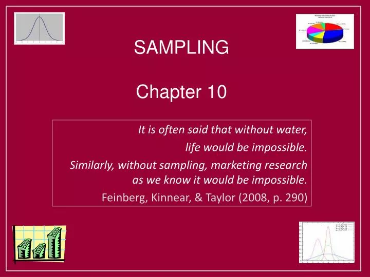
SAMPLING Chapter 10. It is often said that without water, life would be impossible. Similarly, without sampling, marketing research as we know it would be impossible. Feinberg, Kinnear , & Taylor (2008, p. 290). Probability vs. Nonprobability Sampling. Probability Sampling

E N D
SAMPLING Chapter 10 It is often said that without water, life would be impossible. Similarly, without sampling, marketing research as we know it would be impossible. Feinberg, Kinnear, & Taylor (2008, p. 290)
Probability vs. Nonprobability Sampling • Probability Sampling • Each sampling unit has a known probability of being included in the sample • Nonprobability sampling • When the probability of selecting each sampling unit is unknown
Probability Sampling Procedures • Simple Random Sampling • A sampling approach in which each sampling unit in a target population has a known and equal probability of being included • Advantage: Good generalizability and unbiased estimates • Disadvantage: must be able to identify all sampling units within a given population; often, this is not feasible • Systematic Random Sampling • Similar to random sampling, but work with a list of sampling units that is ordered in some way (e.g., alphabetically). • Select a starting point at random, then survey each nth person where the “skip interval” = (population size/desired sample size) • Advantage: quicker and easier than SRS • Disadvantage: may be hidden “patterns” in the data
Probability Sampling Procedures • Stratified Random Sampling • Break up population into meaningful groups (e.g., men, women), then sample within each “strata”, then combine • Proportionate stratified sampling: here you sample based on the size of the populations (i.e., sample more from the bigger strata: e.g., Caucasians) • Disproportionate stratified sampling: sample the same number of units from each strata, regardless of the strata’s size in the pop. • A variant is optimal allocation: here you use smaller sample sizes for strata within which there is low variability (as the lower variability will give you more precision with lower N). • Advantages: more representative; can compare strata • Disadvantages: Can be hard to figure out what to base strata on (Gender? Ethnicity? Political party?)
Probability Sampling Procedures • Cluster Sampling • Similar to stratified random sampling, but with stratified random sampling, the strata are thought to possibly differ between strata (men vs. women), but be homogeneous within strata. • In cluster sampling, you divide overall population into subpopulations (like SRS), but each of those subpopulations (called “clusters”) are assumed to be mini-representations of the population (e.g., survey customers at 10 Red Robins in WA). • Area sampling: clusters based on geographic region
Probability Sampling Procedures • Cluster Sampling • One-step clustering: just select one cluster (e.g., one store); problem = may not be representative of population • Two-step cluster sampling: break into meaningful subgroups (Red Robins in big cities vs. Red Robins in suburbs), then randomly sample within each of those clusters • Advantages: easy to generate sampling frame; cost efficient; representative; can compare clusters • Disadvantages: must be careful in selecting the basis for clusters; also, within clusters, often little variability (they’re homogeneous), and this lack of variability leads to less precise estimates
Nonprobability Sampling Procedures • Convenience Sample • Survey people based on convenience (e.g., college students) • Advantage: is fast and easy • Disadvantage: may not be representative • Judgment Sampling • Use your judgment about who is best to survey • Advantage: Can be better than convenience if judgment is right • Disadvantage: but if judgment wrong, may not be representative/generalizable
Nonprobability Sampling Procedures • Quota Sampling • Sample fixed number of people from each of X categories, possibly based on their relative prevalence in the population • Advantage: Can ensure that certain groups are included • Disadvantage: but b/c you aren’t using random sampling, generalizability may be questionable • Snowball Sampling • You contact one person, they contact a friend (e.g., one cancer survivor is in contact with other survivors, and so recruits them) • Advantages: can make it easier to contact people in hard to reach groups • Disadvantage: there may be bias in the way people recruit others
Factors Affecting Choice of Sampling Procedure • Use some type of random sampling if: • You are collecting quantitative data that you want to use to arrive at accurate generalizations about population • You have sufficient resources and time • You have a good sense for the population • You are sampling over a broader range (e.g., of states, nations)
Computing the Sample Size Based on Usable Rates • Several factors can reduce your sample size • Thus, you may want to plan for more than your final sample size (i.e., use a higher “number of contacts” to achieve your final sample size). You adjust using the following three factors: • RR = reachable rate (e.g., how many people on a telephone list will you actually be able to reach?) • OIR = overall incidence rate (i.e., % of target population that will qualify for inclusion; e.g., can’t use people over 40) • ECR = expected completion rate (i.e., some folks won’t complete your survey) • For example
Computing the Sample Size Based on Usable Rates • You want a sample size of n = 500 • You figure you can reach 95% of the folks on your list (RR = .95) • You think 60% will be 40 or younger (OIR = .60) • You predict that 70% will complete your survey (ECR = .70) • Based on these numbers, you should contact 1,253 people
Some Key Terms • Sampling • Selection of a small number of elements from a larger defined target group of elements and expecting that the information gathered from the small group will allow judgments to be made about the larger group • Population • The identifiable set of elements of interest to the researcher and pertinent to the information problem • Defined Target Population • The complete set of elements identified for investigation • Element • A person or object (e.g., a firm) from the defined target population from which information is sought • Sampling Units • The target population elements available for selection during the sampling process • Sampling Frame • The list of all eligible sampling units
Some Key Terms • Total Error = Sampling Error + Nonsampling Error • Sampling Error • Any type of bias that is attributable to mistakes in either drawing a sample or determining the sample size • Nonsampling Error (controllable) • A bias that occurs in a research study regardless of whether a sample or a census is used (recall all the different types of errors we discussed) • Respondent Errors (non response, response errors) • Researcher’s measurement/design errors (survey, data analysis) • Problem definition errors • Administrative errors (data input errors, interview errors, poor sample design)
Central Limit Theorem • A theory that states that, regardless of the shape of the population from which we sample (e.g., positively skewed), as long as our sample size is > 30, the sampling distribution of the mean (x-bar) will be normally distributed with the following characteristics: The mean of the sampling distribution of the mean will equal the mean in the population. The standard error of the sampling distribution of the mean will equal sample standard deviation (s) divided by sample size (n). This is a sample estimate of the true standard error in population. The larger the sample size, the more precise we can get about our estimate of the true mean in the population (e.g., in our confidence interval).
variance Note: Dr. Joireman does not put a “bar” above s or s2.
Computing Standard Deviation Assume your data are continuous (i.e., are not just yes/no data). For example, let’s say we want to know how much people would be willing to pay for a tennis racquet. We sample 7 folks and wish to generalize to the population…. Results
Formulas forVariance and Standard Deviation Sum of Squared Deviations POPULATION SAMPLE
Highlights Concept Tells a Story “Crank it Out” Faster, Less Meaningful The Sum of Squared Deviations (SS) • Both Formulas Give Identical Answers! • SS = NUMERATOR of the Variance • Examples on board…
This is the “standard deviation” of the sampling distribution of means. This (4.09) will naturally be smaller than our sample standard deviation (10.82) based on our single sample of scores, and it will become smaller as n increases.
Confidence Intervals A confidence interval is the statistical range of values within which the true value of the target population parameter is expected to lie.
Computing Confidence Intervals • 95% Confidence Interval: • We are 95% confident that the mean of the population from which we took our sample has a mean between these lower and upper limits. • To compute, we need: Critical Z-value for our desired level of confidence (see next page for Z-critical values) Standard error of mean Mean of our sample Based on these results, we are 95% confident that the mean in the population from which we sampled is between 66.98 and 83.02. Cool beans!
Common Z-Critical Values • To be 90% confident, you use a z-critical value of 1.65 • To be 95% confident, you use a z-critical value of 1.96 • To be 99% confident, you use a z-critical value of 2.58 An example… Z-critical values for 95% confidence (put ½ of .05 on each side) .025 .025 -1.96 +1.96
What if my data are Yes/No?Here we want to estimate the population percentage. For example, a CNN poll (9/25/08) asked whether readers believed Obama and McCain should continue with their plans to debate on Friday (9/26/08). Results
Recent Poll on Presidential Debate Yes = 75% (or yes, but debate on economy) No = 25% No (wait till bailout is taken care of) N = 9782 Let’s compute standard error and 95% confidence interval Here, p = % yes, q = (1-p) or % no