Journal of Geology & Geophysics

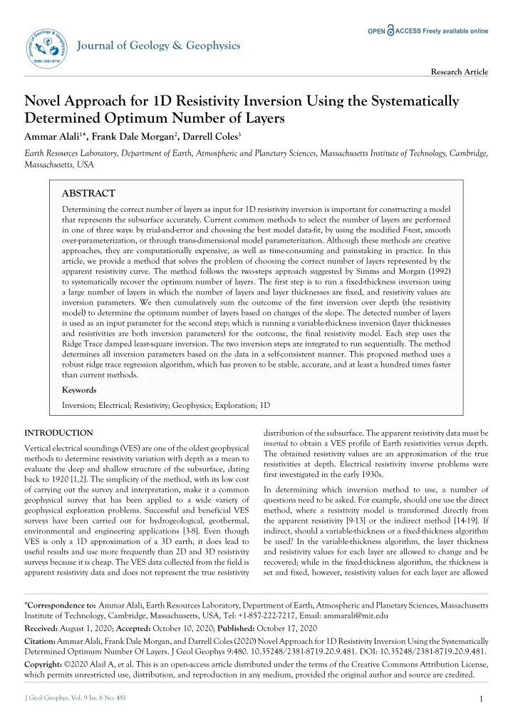
1. ACCESS Freely available online OPEN JournalofGeology&Geophysics ISSN: 2381-8719 Journal of Geology & Geophysics Research Article Novel Approach for 1D Resistivity Inversion Using the Systematically Determined Optimum Number of Layers Ammar Alali1*, Frank Dale Morgan2, Darrell Coles3 Earth Resources Laboratory, Department of Earth, Atmospheric and Planetary Sciences, Massachusetts Institute of Technology, Cambridge, Massachusetts, USA ABSTRACT Determining the correct number of layers as input for 1D resistivity inversion is important for constructing a model that represents the subsurface accurately. Current common methods to select the number of layers are performed in one of three ways: by trial-and-error and choosing the best model data-fit, by using the modified F-test, smooth over-parameterization, or through trans-dimensional model parameterization. Although these methods are creative approaches, they are computationally expensive, as well as time-consuming and painstaking in practice. In this article, we provide a method that solves the problem of choosing the correct number of layers represented by the apparent resistivity curve. The method follows the two-steps approach suggested by Simms and Morgan (1992) to systematically recover the optimum number of layers. The first step is to run a fixed-thickness inversion using a large number of layers in which the number of layers and layer thicknesses are fixed, and resistivity values are inversion parameters. We then cumulatively sum the outcome of the first inversion over depth (the resistivity model) to determine the optimum number of layers based on changes of the slope. The detected number of layers is used as an input parameter for the second step; which is running a variable-thickness inversion (layer thicknesses and resistivities are both inversion parameters) for the outcome, the final resistivity model. Each step uses the Ridge Trace damped least-square inversion. The two inversion steps are integrated to run sequentially. The method determines all inversion parameters based on the data in a self-consistent manner. This proposed method uses a robust ridge trace regression algorithm, which has proven to be stable, accurate, and at least a hundred times faster than current methods. Keywords Inversion; Electrical; Resistivity; Geophysics; Exploration; 1D INTRODUCTION distribution of the subsurface. The apparent resistivity data must be inverted to obtain a VES profile of Earth resistivities versus depth. The obtained resistivity values are an approximation of the true resistivities at depth. Electrical resistivity inverse problems were first investigated in the early 1930s. Vertical electrical soundings (VES) are one of the oldest geophysical methods to determine resistivity variation with depth as a mean to evaluate the deep and shallow structure of the subsurface, dating back to 1920 [1,2]. The simplicity of the method, with its low cost of carrying out the survey and interpretation, make it a common geophysical survey that has been applied to a wide variety of geophysical exploration problems. Successful and beneficial VES surveys have been carried out for hydrogeological, geothermal, environmental and engineering applications [3-8]. Even though VES is only a 1D approximation of a 3D earth, it does lead to useful results and use more frequently than 2D and 3D resistivity surveys because it is cheap. The VES data collected from the field is apparent resistivity data and does not represent the true resistivity In determining which inversion method to use, a number of questions need to be asked. For example, should one use the direct method, where a resistivity model is transformed directly from the apparent resistivity [9-13] or the indirect method [14-19]. If indirect, should a variable-thickness or a fixed-thickness algorithm be used? In the variable-thickness algorithm, the layer thickness and resistivity values for each layer are allowed to change and be recovered; while in the fixed-thickness algorithm, the thickness is set and fixed, however, resistivity values for each layer are allowed *Correspondence to: Ammar Alali, Earth Resources Laboratory, Department of Earth, Atmospheric and Planetary Sciences, Massachusetts Institute of Technology, Cambridge, Massachusetts, USA, Tel: +1-857-222-7217, Email: ammarali@mit.edu Received: August 1, 2020; Accepted: October 10, 2020; Published: October 17, 2020 Citation: Ammar Alali, Frank Dale Morgan, and Darrell Coles (2020) Novel Approach for 1D Resistivity Inversion Using the Systematically Determined Optimum Number Of Layers. J Geol Geophys 9:480. 10.35248/2381-8719.20.9.481. DOI: 10.35248/2381-8719.20.9.481. Copyright: ©2020 Alail A, et al. This is an open-access article distributed under the terms of the Creative Commons Attribution License, which permits unrestricted use, distribution, and reproduction in any medium, provided the original author and source are credited. J Geol Geophys, Vol. 9 Iss. 6 No: 481 1

2. Alali A, et al. ACCESS Freely available online OPEN function. An interested reader is referred to the aforementioned work. to change and be recovered. Lastly, what is the optimum number of layers to be used [20-22] have discussed the answer for the first question and demonstrated that the indirect approach yields better results. Therefore, an indirect method using a nonlinear least- squares inversion is used in this article. Inversion In geophysical inverse problems, the goal is to construct the distribution of subsurface properties (an “earth model”) from measurements usually acquired at the surface. Here, the acquired apparent resistivity curve from the field is inverted to obtain the number of layers, the layer thicknesses, and the electrical resistivity values of horizontal layers sensed by the survey. The work showed that the “variable parameter scheme” inversion, where layer thicknesses and resistivities are inversion parameters, gives the most accurate inversion results [20]. In the “variable parameter scheme,” layer thicknesses and resistivity are inversion parameters, allowed to change and are recovered. The ‘variable parameter scheme’ will be referred to as “variable-thickness inversion” from now on. In this scheme, the optimal number of layers sensed by the electrical survey, which is usually not known before the inversion, is a critical input parameter to represent the sub-surface in the most accurate, yet simple way possible. There exist some methods to estimate the number of layers, such as the F-test, picking the model with lowest calculated error, or by trans-dimensional inversion [20,27,28,30]. It is worth noting that increasing the number of layers means increasing the number of inversion parameters, which usually results in an inversion with less data misfit. However, this does not necessarily best represent the subsurface, for the decreased calculated error is just a by-product of the increase in number of parameters [20]. Thus, some of these methods that depend on the lower calculated error can fail in detecting the optimum number of layers, where the optimum number of layers is the least number of layers with the best data misfit. Also, these methods are time consuming [27]. In the indirect method case, a variable-thickness or fixed-thickness scheme can be followed. In the fixed-thickness scheme, holding the layer thicknesses fixed reduce the number of parameters and the inversion then involves solving only for the layer resistivity values, have used fixed-thickness schemes [23-25]. However, It is demonstrated by examples that the variable-thickness inversion scheme gives the most accurate inversion results that represent the subsurface [20]. Inverting the apparent resistivity data to obtain a resistivity model using the variable-thickness inversion entails a prior selection of the number of layers and many other inversion parameters [20]. Consequently, one can obtain different models for the same input apparent resistivity [26]. Currently, there are few means to determine the number of layers represented by the apparent resistivity data collected. Most commonly, the number of layers is an arbitrary defined parameter in the inversion, and the processor tends to a follow trial and error technique to determine the optimum number of layers. A second method follows the modified F-test as discussed [20]. One additional method to determine the optimum number of layers is trans-dimensional model parameterization [27]. This approach is an extension of Bayesian parameter estimation that accounts for the posterior probability of how complex an earth model is (specifically, how many layers it contains). Each of the methods mentioned above require tens of trials to reach a final conclusion on the optimum number of layers, which is computationally expensive and can take a while to finalize [20,27,28]. Although these methods are creative approaches, they are time-consuming and painstaking in practice. Here, a novel two-step approach for 1D resistivity inversion is adopted. This approach is an extension and simplification of the work done by Simms and Morgan [20]. The proposed method yields a final result of the inversion (number of layers, layer thicknesses, and resistivity values) in one run, which consists of two consecutive steps. The method can be deployed in the field to process the data on the spot and get immediate results. The steps in the proposed methods, as shown in Figure 1, are: The method proposed in this article systematically determines the number of layers used in a VES inversion and takes less than one minute to complete. Therefore, saving the processor time and effort. The method follows the two-step approach suggested to systematically recover the optimum number of layers [20]. Unlike others, this approach has the advantage of allowing the geophysicist to process immediately the data at the field site as it does not require high computational power and can run in a short time. In addition, it is self-consistent, and stable in terms of the convergence of the inversion algorithm. 1. Perform a fixed-thickness inversion in which a large number of layers and their thicknesses are set and fixed at the beginning and only resistivity values are allowed to change and be solved for. METHODOLOGY 2. Obtain the model resistivity profile resulting from the first step. The purpose of the VES inversion is to determine a model of resistivity as a function of the depth of the subsurface. The result of this inversion will be number of the layers and the estimated resistivity and the thickness of each layer. The data collected from the field is the apparent resistivity following different possible configurations [2]. In this article, we will address inverting the data following a novel approach. We will convert the apparent resistivity data to an inverse model using an iterative inversion scheme. The forward model is an essential part of every inversion scheme. 3. Cumulatively sum this resistivity model over depth (resulting in a summation of resistivities over depth). This will be referred to as integrated curve. 4. Determine the number of layers from the points of changing slope in the integrated (cumulative summation over depth) curve, as in Figure 2. 5. Use the number of layers, so determined, for a variable- thickness inversion. In this step, the thickness for each layer is allowed to change simultaneously and be resolved along with the resistivity values. Forward model The forward resistivity modeling code adopts the analytic solution for multiple horizontal resistivity layers reported [2,29]. The apparent resistivity curve (apparent resistivity vs. separation) is computed for a given number of layers, layer thicknesses, and electrical resistivity values of horizontal layers through a kernel The first step of this process is the fixed-thickenss inversion. Initial values are set and fixed for thickness of layers, 1meter. The number J Geol Geophys, Vol. 9 Iss. 6 No: 481 2

3. Alali A, et al. ACCESS Freely available online OPEN Figure 1: Breakdown of the two-step approach. Figure 2: Graphic illustration of integrated resistivity curve (resulted of cumulatively summing the resistivity values over depth) of a fixed-layer resistivity model. The horizontal axis is the integrated resistivity values and the vertical axis is depth. The points of changing slope at depth 10, 15, and 25 m are layer boundaries. The number of layers detected here is three layers plus the half space at the bottom. The number of layers, three in this example, will be used as the number of layers in the next step of the inversion, variable-thickness inversion. The points of changing slope indicate layer boundaries and will be used as initial values for layer thicknesses in the variable-thickness inversion (10, 5, and 10 m layer thicknesses). of layers equals the total depth and is not allowed to change. The resistivity values can vary and are solved [20]. The purpose of fixing the layer thicknesses is to reduce the parameters solved for during the inversion process to resistivity values only. By doing this, non-uniqueness may be reduced [20], because of the resistivity thickness product can be recovered [31]. The resulting resistivity model is then cumulatively sum over depth to create an “integrated resistivity” curve. The purpose of integrating the resistive model is to smooth the small changes over depth and only those significant changes from the resistivity model will be pronounced as a change of slope on the integrated curve. The slope at each point in the curve is calculated (f’(x)), and the point of changing slope will be interpreted for a layer boundary that represents a new layer in the model with a different ‘true’ resistivity value, as illustrated in Figure 2. These points of changing slope in the integrated curve correlate with the inflection points in the resulted resistivity model from the fixed-thickness inversion (f’’(x)=0), as shown later. though they are allowed to change during the variable-thickness inversion, can be a good first guess for a faster convergence. In the variable-thickness inversion, layer thicknesses and resistivity values are each allowed to change and be solved. This scheme guarantees that the number of layers is not an arbitrary guess, but a systematically determined parameter. The inversion scheme used is a damped non-linear least square (NLLS). The modeled parameters X describing the system is related to observed data b through the forward model operator such that: . (1) The main objective in the inversion is to determine parameters from the observed data b. The lowest data misfit exists with the minimum difference between the observed data (field data) and the modeled data (calculated data). A common method used to quantify the misfit between observed and model data is the Root Mean Square Error, which is also known as RMSE. Minimizing the RMSE is achieved by providing a least square solution for Equation (1). This solution is provided by a correction vector updated at each iteration [33]: Simms and Morgan explained that the number of layers is usually based on the shape of the sounding curve (apparent resistivity curve), but can hide either thin layers and/or an adjacent layer with a small contrast of resistivity [20]. However, the proposed method is sensitive to thin layers and changes of resistivity. Figure 2 illustrates how the number of layers is calculated based on the layer boundaries detected from this curve. This method assumes that each layer with a resistive value will be represented with constant accumulating rate, which will be reflected as constant slope on the integrated curve. The points of change of the slope (f’(x)) will be considered as a new layer with a new resistivity value. This is a stable method to obtain the optimal number of layers that can represent the subsurface [32]. This number of layers is then used as input for the variable-thickness inversion and the depths of the layer boundaries are used as initial values for the layer thicknesses as shown in Figure 2. Using the layer boundaries as initial values for the layer thicknesses, even , which is (2) Where Jacobian matrix, and is the correction vector to the parameters , is data misfit. is the However, calculating the inverse in equation (2) can be computational expensive, or impossible if matrix. To avoid these problems, we will follow a damped NLLS method. Equation (2) will become: is a singular (3) Where is a simple regularization parameter (“damping”) and I is the identity matrix. In order to further stabilize the Jacobian matrix, we will apply correlation-rescaling [34]. J Geol Geophys, Vol. 9 Iss. 6 No: 481 3

4. Alali A, et al. ACCESS Freely available online OPEN is arriving to a convergence stage of 99.5% that satisfies this condition [33]: Correlation Rescaling Correlation rescaling is a method to stabilize the inversion of the Jacobian matrix. After the data is conditioned by correlation rescaling, the range for the regularization parameter is between 0 and 1. Let’s redefine [33,34]: (13) The same inversion algorithm and same the fixed-thickness and variable-thickness inversions. We use the latter method. are applied for .(4) (5) RESULTS . (6) Synthetic examples Define Model studies with established and known solutions enable researchers to realistically evaluate inversion methods. Several synthetic models have been computed and inverted to validate the inversion scheme. The first synthetic example follows a Schlumberger configuration with a simple and shallow model. The second example also follows a Schlumberger configuration but with a deeper and more complex model that includes both resistive and conductive layers. Finally, the third example follows a Wenner configuration. In the synthetic examples, the following parameters are controlled: number and location of measurements, number of layers in the subsurface, layers thicknesses, and true resistivities. The forward 1D resistivity model is used to create the synthetic data of apparent resistivities using input parameters, as explained previously. From the apparent resistivity and the survey geometry, the layers thicknesses and resistivities are inverted for. . (7) . (8) Then the original correctional vector in equation (2) will be: . (10) After the conditioning, the matrix is stable and the damping value is limited between 0 and 1. Picking the right damping value will lead to fast convergence but also stable algorithms. To ensure self- sufficiency that is stable and will always converge, we will run the Ridge Trace algorithms to pick the damping value [35]. Ridge trace regression We have discussed adding a damping factor to help obtain an inverse for the matrix in equation (2). Also, by adding the damping factor , we accept a little bias, and substantially reduce the variance, thereby improving the mean square error of the estimation [35]. The Ridge Trace algorithm is used to decide the value. It is stable in terms of convergence, with one adjustable parameter, , that results in an optimal damping factor. The algorithm determines which damping value to use for each parameter individually. This method provides a damping matrix instead of a single damping value for all inversion parameters. The algorithm provides NLLS solutions for a range of damping values between 0 and 1, and calculates the gradient for each parameter [35]: Case 1: Schlumberger Configuration –Simple Model The first example is a simple and shallow two-layer model where the resistivity increases as a function of depth. Table 1 shows the input parameters (points of measurements, number of layers, layer thicknesses, and true resistivity values). The input parameters are used to generate the apparent resistivity curve using the forward model. Typically, a maximum current electrode spacing needs to be three times the depth of investigation to guarantee sufficient data [36,37]. The resistivity values are for layer-1, layer-2, and a half space. The used data consists of the current electrodes spacing L, the potential electrodes spacing and apparent resistivity. Figure 3 shows a plot of the apparent resistivity curve. The apparent resistivity plot contains half-current electrodes spacing Land the apparent resistivity at that point. (11) Figure 4 presents the first step of the inversion, the fixed-thickness inversion. The inversion will run without any additional input and determine the resistivity value bounds from the apparent resistivity provided in the imported data. In Figure 5, the top plot shows the RMS error. The bottom-left plot shows the data and inverted fit, with quantified RMSE that changes per iteration. The bottom- right plot shows the resistivity as a function of depth. Note that it is hard to determine the number of layers and their depths with any accuracy from the apparent resistivity VS depth plot in Figure 4. The fixed-thickness inversion will supply us with a resistivity model as shown in the bottom right of Figure 4. This resistivity model is integrated and used in the next step for detecting the number of layers covered by this survey. Figure 5 shows the result of cumulatively summing this resistivity model. In Figure 5, the number of layers can be visually estimated to be two by counting the sharp changes along this curve. There is an automated process in place to detect the number of layers from the curve based on the changes of the slope. So, the slope changes (blue starts) are detected automatically as the slope of the curve changes value. The number of layers is used as input for the variable-thickness inversion. For each parameter, the damping per iteration is the minimum for which . The can result in a smooth convergence. The damping value is chosen right before the parameter starts to rapidly diverge, which will be shown later by examples. It is worthy to note that the inversion cannot handle the addition of data uncertainty, and assumes that data uncertainties are normal with a mean of 0 and a standard deviation of 1. With each iteration i, the parameters are updated and a forward model is run to compare the modeled and observed apparent resistivities and a root mean square error (RMSE) is calculated: is set at 0.4, a value that . (12) Where: =1,2,..,n n is the number of data points. di is the residual between data and model. The solution will continue to converge per iteration until it satisfies a stopping mechanism. One stopping mechanism is the number of iterations; the inversion will stop when it reaches the maximum iteration number, 150. The other stopping mechanism J Geol Geophys, Vol. 9 Iss. 6 No: 481 4

5. Alali A, et al. ACCESS Freely available online OPEN Table 1: Input parameters for case 1. Type ρ [Ω·m] Thickness [m] Input 100, 150, 200 5,7, ∞ 9 Number of measurements (expand electrode separations logarithmically) Figure 3: Plot of the apparent resistivity for case 1. The x-axis is the apparent resistivity, and the y-axis is half current electrodes spacing. The 9 points of apparent resistivity show trend of increased resistivity with depth. Figure 4: Fixed thickness inversion for case 1. The top section shows RMSE at each iteration. Bottom left is data and inverted fit. Bottom right is the resistivity model. The changes of the slope in the curve (shown in Figure 5) correlate with the inflection points of the resistivity model from the fixed- thickness inversion. However, based on many trials, using the integrated curve is a more stable method to select the number of layers than using the inflection points in the resistivity model, lower left of Figure 4, and it also mutes the noise. Figure 6 shows a comparison between the detected layer boundaries, derived from the “integrated fixed-thickness resistivity model,” and the actual boundaries from the synthetic model. In this comparison, we multiply the fixed-thickness resistivity model by ten to be able to plot it on the same scale. The last two points of the resistivity profile representing the last layer were neglected, as it is usually poorly recovered because the last layer is not bounded by anything underneath it. From Figure 7, the reader can see how the detected layer boundaries (green) correlates with the change of slopes in the integrated resistivity profile (red) and the inflection points in resistivity model resulted from the fixed-thickness inversion (blue). The true layer boundaries (grey) are from the synthetic model. J Geol Geophys, Vol. 9 Iss. 6 No: 481 5

6. Alali A, et al. ACCESS Freely available online OPEN Figure 5: Integrated resistivity model for case 1. The blue stars indicate the start of each new layer. The number of layers detects is two. Figure 6: Comparison between the detected layer boundaries, derived from the “integrated fixed-thickness resistivity model,” and the actual boundaries from the synthetic model for case 1. The number of layers detected (two layers) is used as an input for the variable-thickness inversion. Also, the depths of layer boundaries, detected at 5 m and 12 m, are used as initial values for layer thicknesses (5 m and 7 m). In this case, it happened to be the exact match between the detected layer boundaries and the true layer boundaries from the synthetic model. However, this is not always the case, as the reader will see in the next example. Therefore, in the variable-thickness inversion, both layer thickness and resistivity values are allowed to change and be recovered. Figure 8 shows the variable-thickness inversion. This is the last step of the inversion and the final resistivity model is shown at the bottom-right of Figure 7. Figure 8 shows a comparison between the synthetic and the inverted model. The same step. The final result of the variable-thickness inversion has data RMSE of 0.00%. Figure 9 shows almost a perfect match between the synthetic and inverted models. Table 2 compares the input and inverted model parameters for case 1. Case 2: Schlumberger Configuration Table 3 shows the input parameters used to generate the apparent resistivity curve following the Schlumberger configuration. This is a three-layer model with two resistive layers on top of a less resistive layer and a half space. Even though having higher resistivity contrast is between layers is easy to detect, the higher contrast makes it difficult for the inversion to determine the true resistivity values and layer thickness esaccurately and independently [20,31]. I will use these parameters to synthesize a noise-free apparent resistivity following the forward model. Figure 9 shows the resulting apparent resistivity curve for the parameters given in Table 3. The result of the forward model is used as in the previous J Geol Geophys, Vol. 9 Iss. 6 No: 481 6

7. Alali A, et al. ACCESS Freely available online OPEN Figure 7: The result of the variable-thickness inversion. The bottom-right plot states the number of layers used in title, and the half-space (last layer in the resistivity model) is shown in dashes. Figure 8: Comparison between the synthetic and inverted model for case 1. is used as an input for the inversion. The inversion will run without any additional input. The both steps of inversion (fixed-thickness and variable-thickness inversion). Figure 10 shows the fixed-thickness inversion. as initial values for layer thicknesses. The points of changing slope are classified as new layer boundaries. Those points of changing slope on the integrated resistivity curve correlate with inflection points in the fixed-thickness resistivity model. Figure 12 shows the comparison between the detected layer boundaries, derived from the “integrated fixed-thickness resistivity model,” and the actual boundaries from the synthetic model. In order to plot both the “fixed-thickness resistivity model” and the “integrated resistivity model” on the same scale, we multiplied the values of the former by twenty. is set at 0.4 for In Figure 11, the number of layers can be visually estimated to be three via counting the sharp changes along this curve. The same mechanism discussed before is implemented here to detect the number of layers (three layers plus half space). Once satisfied with the result, the number of layers is used as input for the variable- thickness inversion, and the depth of layer boundaries are used J Geol Geophys, Vol. 9 Iss. 6 No: 481 7

8. Alali A, et al. ACCESS Freely available online OPEN Figure 9: Plot of the current electrode spacing (AB/2) and apparent resistivity values for the 18 measurements, case 2. Table 2: Input and inverted parameters for case 1. Type ρ [Ω·m] Thickness [m] Data RMSE Input Output 100, 150, 197 5, 6.5, ∞ 0.00% 100, 150, 200 5, 7, ∞ - Table 3: parameters for case 2. Type ρ [Ω·m] Thickness [m] Input 1000, 2000, 200, 500 10, 20, 30, ∞ 18 Number of measurements (expand electrode separations logarithmically) Figure 10: Fixed-thickness inversion for case 2. The top shows data RMSE per iteration. Bottom left is the data and inverted fit with RMSE. Bottom right is the resistivity model. J Geol Geophys, Vol. 9 Iss. 6 No: 481 8

9. Alali A, et al. ACCESS Freely available online OPEN Figure 11: The integrated resistivity for case 2. Stars indicate the points where a new layer is detected. Figure 12: Comparison between the detected layer boundaries, derived from the “integrated fixed-thickness resistivity model,” and the actual boundaries from the synthetic model for case 2. The match between the detected layer boundaries and the true layer boundaries (based on the synthetic model) increases in error with depth as shown in Figure 12. Using the extracted number of layers, the next step of variable-thickness inversion starts with using the number of layers (three layers) and the initial values of the layer thicknesses (11 m, 20 m, 49 m). The initial values of layer thicknesses are good preliminary guesses for faster convergence, but the layer thicknesses are allowed to change during the variable- thickness inversion and recovered along the resistivity values. Figure 13 shows the result of the variable-thickness inversion. This is the last step of the inversion and the resulting final resistivity model is shown at the bottom-right of Figure 13. The final resistivity model presents layer thicknesses different from the initial values, as both layer-thicknesses and resistivity values are recovered. In an effort to simulate more realistic data conditions, we added different levels of Gaussian noise (5% and 20%) on the apparent resistivity points on the same example of case 2 While the scheme was able to detect the number of layers for each of the added noise cases (three layers plus half space), the variable- thickness inversion resulted in higher data RMSE, as expected, in comparison to the case with no added noise. Figure 14 shows a comparison among the synthetic model, the inverted model with no noise, the inverted model with 5% Gaussian noise, and the inverted model with 20% Gaussian noise. Table 4 compares the input parameters, the inverted parameters of the previous case with J Geol Geophys, Vol. 9 Iss. 6 No: 481 9

10. Alali A, et al. ACCESS Freely available online OPEN Figure 13: The result of the variable-thickness inversion. Bottom-right plot's title states the number of layers used, the half space is shown in dashes. Figure 14: Comparison of the synthetic (data), the inverted model with no noise, and the inverted model with different levels of added noise, case 2. Table 4: Comparison between input parameters, inverted parameters without noise and with added noise. Type ρ [Ω·m] Thickness[m] Data RMSE Input Output for case without noise 999, 2017, 173, 789 10, 19.8, 29.6, ∞ 0.05% Output for case with 5% noise 1,00,32,03,51,63,850 10, 19.7, 29.5, ∞ 0.08% Output for case with 20% noise 1,00,02,00,71,65,970 10, 20.2, 29.2, ∞ 0.20% 1000, 2000, 200, 500 10, 20, 30, ∞ - no noise, and the inverted parameter with a different percentage of added Gaussian noise. The final inverted resistivity models are better match to the synthetic model at the shallow part than it is with the deeper portion. This results from a reduction in the recovering power of resistivity sounding data with increasing depth [20,27,31]. While a higher contrast between the resistivity values (from 2000 Ω·m to 200 Ω·m between layer 2 and layer 3) is easy to detect, it becomes more difficult to recover accurately [20]. As it explains that the recovering power of the resistivity can only recover the resistivity-thickness product (resistive layer) or conductivity- thickness product (conductive layer) [31]. The combination of covering deeper layers and a more complex model (higher contrast of resistivity values between layers) lower the resolving power and that is reflected by the model error, especially at the last two layers as shown in Figure 15. The output of the inversion (resistivity model) with 5% and 20% added Gaussian noise is relatively good J Geol Geophys, Vol. 9 Iss. 6 No: 481 10

11. Alali A, et al. ACCESS Freely available online OPEN Figure 15: Elevation map with sounding locations along the Roseau 10 line (Morgan et al., 2013). with calculated data RMSE less than 1%. Even though the added Gaussian noise to the apparent resistivity points is 5%, the lower RMSE is an indication of how the inversion results are more a function of how unique the solution rather than how much noise it has [20]. Simms and Morgan (1992) go on to explain how in 1D resistivity, problems with equivalence are so dominant that the errors in parameters are due mainly to uniqueness and resolution aspects (which are controlled mainly by depth and contrast between resistivity values as explained in the previous sections), and not to the random noise in the data. chargeability was created. A normalized chargeability value close to zero indicates a near clay-free zone [41]. A curious reader is referred to the listed citations [39-42]. In this article, however, we will only focus on the resistivity data. In order to interpret the resistivity data, we use Archie’s law, an empirical formula relating measured ground resistivities to the porosity and the resistivities of pore water [43]. Archie’s empirical law was used to determine the effective electrical conductivity of the groundwater within the Roseau watershed. Resistivity values ranging from 200-3000 Ω·m were considered to be water-bearing geological material based on Archie’s law. Field data example: Roseau (vanard) watershed, saint lucia Site selection The data used in this section is part of fieldwork jointly performed by Frank Dale Morgan (MIT) and members of the Water Resources Management Agency (WRMA) in Saint Lucia in 2014. The primary motivation for this work is to search for a productive groundwater aquifer in Saint Lucia to meet the growing demand for drinking water on the island and to find a reliable water source for use in times of emergency. One of the most pressing issues affecting Saint Lucia today is a shortage of water. This problem is projected to become increasingly severe with further development and could limit the growth of the island's economy. The study was aimed at conducting geophysical exploration for possible potable groundwater resources in one or two watersheds of Saint Lucia. Groundwater is very resilient to extreme climate conditions and natural disasters such as hurricanes and droughts. The Roseau watershed of North West Saint Lucia was thoroughly investigated. Based on analysis of previous surveys taken in 1985, 2012, and 2013 [44], a decision was made to further explore a site in the Roseau Watershed, called Roseau 10 as shown in Figure 15. The 2014 survey thus aimed to locate regions of relatively high resistivity using geophysical sounding methods in this area. To survey what rock types were underneath the road at Roseau 10 and whether the rocks contained water, a succession of six Schlumberger arrays 1D VES at about 150 m intervals were completed for a total of 900 m (between 10-100 VES to 10-900 VES) as shown in Figure 15. RESULT Originally, the data was processed using inverse methods to determine the 1D resistivity structure that best matched the measured resistivities and minimized the data RMSE. Two 1D inversion software programs were used to generate two separate models of resistivity. The two inversion techniques were: a fixed- thickness inversion with resistivity measurements and a variable- thickness inversion with resistivity measurements. Both the variable- thickness and fixed-thickness inversions assume fundamental homogenous layers. Each technique was tried a number of times to reach the optimum parameters, such as damping factor and number of layers. Here we will reprocess one of the surveys “Roseau 10-600 VES” using the two-step approach explained in this article. The survey was chosen specifically because it is the closest to the recommended drilling site and it reveals a potential site for a groundwater aquifer. The Roseau 10-600 VES was reprocessed using the two-step approach explained in this article is shown in Figures 16-20. The algorithm succeeded in recovering the number of layers (four layers and a half space) and inverting for their thicknesses and resistivity values that are essential for water Field Methods In order to ascertain the hydrogeology of the Roseau watershed, research was conducted on previous studies and geophysical and geological data were collated in order to inform the areas for focused study. Geophysical methods (1D electrical resistivity and induced polarization) were employed for in-field data collection. The data was then analyzed using 1D resistivity and induced polarization inversion codes. Large amounts of clay produce a polarizing effect, which increases the chargeability. The chargeability is a measure of the induced polarization in the subsurface, which is sensitive to the low- frequency capacitance of rocks. Normalized chargeability is defined as the chargeability divided by the resistivity magnitude [38-40]. Using the induced polarization data, a model for the normalized J Geol Geophys, Vol. 9 Iss. 6 No: 481 11

12. Alali A, et al. ACCESS Freely available online OPEN Figure 16: Plot of current electrode spacing (AB/2) and the apparent resistivity for Roseau10-600 VES survey in Saint Lucia with 20 measurements. Note that it is hard here, even harder than the synthetic-data shown before in Figure 3, to detect the number of layers and their depths with any accuracy from the apparent resistivity VS depth plot in Figure 16. Figure 17: Fixed-thickness inversion for Roseau10-600 VES survey in Saint Lucia. Figure 18: The integrated resistivity for Roseau10-600 VES. Visually, four layers can be detected following the sharp changes in the curve, which is exactly what the algorithm detects. J Geol Geophys, Vol. 9 Iss. 6 No: 481 12

13. Alali A, et al. ACCESS Freely available online OPEN Figure 19: The result of the variable-thickness inversion for Roseau10-600 VES in Saint Lucia. Figure 20: The inverted resistivity model for the Roseau 10-600 VES. Figure 21: Variable-thickness resistivity model for Roseau 10-600. The data was processed using a MATLAB code developed at the Earth Resources Laboratory at MIT. The inversion was run many times with a varying number of layers. J Geol Geophys, Vol. 9 Iss. 6 No: 481 13

14. Alali A, et al. ACCESS Freely available online OPEN explorations in that area. Our two-step self-consistent approach can be deployed to process the data immediately in the field. than one minute), compared to several runs needed to reach the final model otherwise, like it was done originally when the data was acquired. (Figure 21) Because the inversion produces a non-unique solution, we will attempt additional analysis to support my findings from the inversion we ran using a four-layer model. The inversion was run several times using different numbers of layers ranging from 1 to 6. Figure 22 shows a comparison among the inverted models, the apparent resistivity curves and fits, and the associated data RMSE. The result shows a significant drop in the data RMSE between the one-layer and the two-layer model. It further shows that the data RMSE continues to drop slightly as the number of layers increases until it reaches the lowest data RMSE of 4.58% at the four- and five-layer models. However, the four-layer model represents the least number of layers with the lowest data RMSE. This finding confirms the previous choice of four as the optimum number of layers for the inversion. The final inverted model is based on four layers and a half space with data RMSE of 4.58%. From the resistivity data presented in Figure 20, there appears to be four layers of sediments that extend to a depth of 113 m. The first layer has a low resistivity of 8.6 Ω·m, then the resistivity increases in the second layer to 65.9 Ω·m, and drops after that to 28.03 Ω·m. These low resistivity values can be interpreted to indicate a high proportion of clay. Below 113 m, andesite bedrock, the resistivity jumps to 400 Ω·m, which is within our interest area of resistivity. In order to interpret the resistivity model we use Archie’s law to estimate the porosity of the rock. The layer of rock below 113 m depth has a resistivity of 400Ω·m. In the absence of clay deposits in this layer (confirmed by the low normalized chargeability), a resistivity value of 400 Ω·m corresponds to porosity values between 30% and 36% according to Archie’s law with the resistivity of water equal to 40-50 Ω·m. Therefore, the layer below 113 m might be a productive aquifer. So, the site with the highest potential for groundwater is at 550 meters along the road (which is by the location of the Roseau10-600 VES) and a depth below 113 meters. It is worth mentioning that no borehole data exists close this area at this time to confirm any of the interpretations. DISCUSSION The problem of equivalence in resistivity inversion is well known. The ability to invert resistivity data successfully depends on the uniqueness of the model. One of the main factors that increase the uniqueness of the model is determining the optimum number of layers represented by the apparent resistivity curve. There exist different methods used in selecting the number of layers in electrical resistivity inversion. One of the common methods is running an inversion many times using different parameters and different numbers of layers, then comparing the results, where the model with the least number of layers and the lowest data RMSE This site location agrees with the final recommendation of the work done by the group in 2014. Although both approaches resulted in similar conclusions, the proposed approach is better in practice as it yields the final result in one run which consists of two steps (less Figure 22: Inversion models (top), data and fit (middle) and data RMSE (bottom) for models from 1 to 6 layers. Apparent resistivity data are for the Roseau 10-600 VES. The data RMSE drops significantly from one-layer to two-layer. The data RMSE continues to drop slightly until it reaches the lowest RMSE for four-layers and five-layers models, then it increases slightly (0.01%) for the six-layer model. J Geol Geophys, Vol. 9 Iss. 6 No: 481 14

15. Alali A, et al. ACCESS Freely available online OPEN is assumed to be the optimal one [20]. However, this method is computationally expensive and can yield conflicting results due to changes in other parameters, such as the damping factor, in the inversion. Another method is the modified F-test following the Bayesian approach which incorporates a penalty with increasing number of layers in order to solve the inverse problem and solves for the number of layers with accumulated error and penalty [20,30]. Yet another method to determine the optimum number of layers is trans-dimensional model parameterization [27]. This approach is an extension of Bayesian parameter estimation that accounts for the posterior probability of how complex an earth model is (specifically, how many layers it contains). Although these methods are creative approaches, they are time-consuming and painstaking in practice. For example, with trans-dimensional model parameterization, it takes an average of three hours to select the optimum number of layers represented by the apparent resistivity curve, making it computationally expensive [27]. REFERENCES 1. Stefanesco S, Schlumberger C, Schlumberger M. On the electrical distribution pot around a pontoon in a ground with horizontal layers, homogeneous and isotopes. J Phys Radium. 1930.7:132–140. 2. Parasnis DS. Principles of applied geophysics. 4th edn, New York, Chapman and Hall. 1980. 3. Batayneh AT, AS AlZoubai, AA Abueladas. Geophysical investigations for the location of a proposed dam in Al Bishriyya (Al Aritayn) area, Northest Badia of Jordan. Environ Geol. 2001.40:918-992. 4. Mota R, RAM Santos, A Mateus, FQ Marques, MA Goncalves, J Figueiras, et al. Granite fracturing and incipient pollution beneath a recent landfill facility as detected by geoelectrical surveys. J Appl Geophy. 2004.57:11-22. 5. Agnesi VM, Camarda C, Conoscenti C, Di Maggio, IS Diliberto, P Madonia et al. A multidisciplinary approach to the evaluation of the mechanism that triggered the Cerda landslide (Sicily, Italy). Geomorphology. 2005.65:101-116. We propose a two-step approach that systematically determines the number of layers in a single run. This method takes the field data (apparent resistivity) as an input and runs a fixed-thickness inversion, where the thickness of each layer is set and fixed a priori. The resulting resistivity model is then integrated. The integrated curve is used to select the number of layers based on the changed slope in the curve. The change of the slope indicates a new region with different true resistivity, which signifies a layer boundary [32]. This Based on the number of layer boundaries, the number of layers is selected. The number of layers is then used in a variable- thickness inversion that outputs the inverted resistivity values and layer thicknesses. This approach is better in practice to select the optimum number of layers. The method is done in one-run and integrated to take the data from the fixed-thickness inversion to the variable-thickness inversion. While one can be tempted to determine the number of layers from the apparent resistivity profile, in practice, it is hard to preciously determine the number of layers and their depths with accuracy just from the apparent resistivity as can be seen in a synthetic-data Figure 3, and in the field-data Figure 16. Another factor in support of the ability to invert resistivity data successfully is the robustness of the inversion algorithm. Here, we use the Ridge Trace algorithm in damped- least square inversion, which provides stability in convergence, and self-consistence in selecting the optimal damping factor for each parameter individually per iteration. 6. Ozurlan G, MH Sahin. Integrated geophysical investigations in the Hisar geothermal field, Demirci, Western Turkey. Geothermics. 2006.35:110-122. 7. Asfahani J, Y Radwan. Tectonic evolution and hydrogeological characteristic of the Khanaser Valley, Northern Syria, derived from the interpretation of the vertical electrical sounding. PURE APPL GEOPHYS. 2007.164:2291-2311. 8. Park YH, SJ Doh, ST Yun. Geoelectric resistivity sounding of riverside alluvial aquifer in an agricultural area at Buyeo, Geum river watershed, Korea: An application to groundwater contamination study. Environ Geol. 2007.53:849-859. 9. Slichter LB. The interpretation of resistivity prospecting methods for horizontal structures. Phys. 1933.4:307–322. 10. Pekeris CL. Direct method of interpretation in resistivity prospecting. Geophys. 1940.5:31–46. 11. Vozoff K. Numerical resistivity analysis-Horizontal layers. Geophys. 1952.23:536–556. 12. Koefoed O. A fast method for determining the layer distribution from the raised kernel function in geoelectrical sounding. GEOPHYS PROSPECT. 1970.18:564–570. 13. Ghosh DP. The application of linear filter theory to the direct interpretation of geoelectrical resistivity sounding measurements. GEOPHYS PROSPECT. 1971.19:192–217. CONCLUSION 14. Flathe H. 1955. A practical method of calculating geoelectrical model graphs for horizontally stratified media. GEOPHYS PROSPECT. 1955.3:268–294. The solution for the electrical resistivity profile with depth from apparent resistivity is non-unique. The work of Simms and Morgan (1992) showed that the “variable parameter scheme,” where layer thicknesses and resistivities are inversion parameters, yields the most accurate inversion results. The variable parameter scheme requires selecting the number of layers a priori [20]. Also, most inversion algorithms require input parameters, which can be arbitrary and increase the uncertainty of the result like the stopping criteria and the damping value. Here, we have provided a robust approach that chooses the inversion parameters and determines an optimum number of layers. This approach is at least a hundred times faster than currently used methods. The damped least squares inversion algorithm uses correlation rescaling of the Jacobian and Ridge Trace regression to ensure robustness of the algorithm and avoidance of singularity [35]. We have selected a as the default value that can achieve a smooth convergence. The method is computationally faster than other methods, and yields a high degree of accuracy. 15. Onodera S. The kernel function in multiple layer resistivity problem. J Geophys. 1960.65:3787–3794. 16. Roman I. The kernel function in the surface potential for a horizontally stratified earth. Geophys. 1963. 28:232–239. 17. Van Dam JC. A simple method for calculation of standard graphs to be used in geoelectrical prospecting. doctoral dissertation, Delft Technological University. 1964. 18. Mooney HM, E Orellana, H Pickett, L Tornheim. A resistivity computation method for layered earth models. Geophys. 1966.31:192–203. 19. Ghosh DP. Inverse filter coefficients for the computation of apparent resistivity standard curves for a horizontally stratified earth. GEOPHYS PROSPECT. 1971.19:769–777. of 0.4 20. Simms JE, FD Morgan. Comparison of four least-squares inversion schemes for studying equivalence in one-dimensional resistivity interpretation. Geophys. 1992.57:1282-1293. J Geol Geophys, Vol. 9 Iss. 6 No: 481 15

16. Alali A, et al. ACCESS Freely available online OPEN 21. Simms JE, FD Morgan. Re-evaluation of Pekeris' I-D resistivity interpretation method. GEOPHYS PROSPECT. 1990.8:130-136. 33. Morgan FD, VN Rama Rao, C Darrell. Data and models in engineering, science and business. 2nd edn. Cambridge, Massachusetts. 2011. 22. Simms JE, Morgan FD. Reply to letter: Direct and indirect methods of one-dimensional resistivity interpretation. GEOPHYS PROSPECT. 1990.6:386. 34. Marquardt DW, Snee RD. Ridge regression in practice. Am Stat. 1975.29:3–20. 35. Hoerl AE, Kennard RW. Ridge regression: Biased estimation for nonorthogonal problems. Technometrics. 1970.12:55–67. 23. Marsden D. The automatic fitting of a resistivity sounding by a geometrical progression of depths. GEOPHYS PROSPECT. 1973.21:266- 280. 36. Apparao A, T Gangadhara Rao. Depth of Investigation in resistivity methods using linear electrodes. 1974.22:211-223. GEOPHYS PROSPECT. 24. Parker RL. The inverse problem of resistivity sounding. Geophys. 1984.49:143-215. 37. Telford WM, Geldart LP, RE Sheriff. Applied Geophysics. 2nd edn., New York, Cambridge University Press. 1990.552-577. 25. Zohdy AAR. A new method for the automatic interpretation of Schlumberger and Wenner sounding curves. Geophys. 1989.54:245- 253. 38. Marshall DJ, Madden TR. Induced polarization: A study of its Causes. Geophys. 1959.24:790-816. 26. Langer RE. On the determination of earth conductivity from observed surface potentials. Bull Am Math Soc. 1936.42:747-754. 39. Keller GV. Analysis of some electrical transient measurements on igneous, sedimentary and metamorphic rocks, in Wait, JR Edn, Overvoltage research and geophysical applications. Pergamon Press. 1959.92–111. 27. Malinverno A. Parsimonious bayesian markov chain monte carlo inversion in a nonlinear geophysical problem. Int J Geophys. 2002.151:675-688. 40. Lesmes DP, Frye KM. Influence of pore fluid chemistry on the complex conductivity and induced polarization responses of Berea sandstone. J Geophys Res. 2001.106:4079-4090. 28. Nazerali, Nasruddin Abbas. Effects of lateral heterogeneity on id d.c. resistivity and transient electromagnetic soundings in Kuwait. M.S. thesis, Massachusetts Institute of Technology. 2015. 41. Slater LD, Lesmes D. IP interpretation in environmental investigations. Geophysics. 2002.67:77–88. 29. Dimri V. Deconvolution and Inverse theory: Application to geophysical problems, methods in geochemistry and geophysics. Elsevier.1992.140-144. 42. Sogade JA, Scira-Scappuzzo F, Vichabian Y, Shi W, Rodi W, Lesmes DP, et al. Induced-polarization detection and mapping of contaminant plumes. Geophys. 2006.71. 30. Box GEP, J Wetz. Criteria for judging adequacy of estimation by an approximating response function. University of Wisconsin, statistics department, technical report no. 1973.9. 43. Archie GE. The electrical resistivity log as an aid in determining some reservoir characteristics. Petroleum Transactions of AIME. 1942.146:54–62. 31. Madden TR. The resolving power of geoelectric measurements for delineating resistive zones within the crust, the structure and physical properties of the earth's crust, Geophys Monogr. 1971.14: 95-105. 44. Morgan FD, Y Agramakova, F Leon, M Engeliste, R Rock, J Ramine, et al. Water resource management agency (wrma) and department of forestry, ministry of sustainable development, energy, science and technology. geophysical exploration for potential groundwater sites in the roseau watershed of st. Lucia. 2013. 32. Israil M, T Pravin, K Gupta, DK. Tyagi. Determining sharp layer boundaries from straightforward inversion of resistivity sounding data. J Ind Geophys Union. 2004.8:125-133. J Geol Geophys, Vol. 9 Iss. 6 No: 481 16