Download
1 / 22
220 likes | 244 Views
Modes of Annular Variability in the Atmosphere and Eddy-Zonal Flow Interactions. 1. Imperial College London, UK 2. National Centre for Atmospheric Science, University of Reading, UK. Sarah Sparrow 1,2 , Mike Blackburn 2 and Joanna Haigh 1.

E N D
Modes of Annular Variability in the Atmosphere and Eddy-Zonal Flow Interactions 1. Imperial College London, UK 2. National Centre for Atmospheric Science, University of Reading, UK Sarah Sparrow1,2, Mike Blackburn2 and Joanna Haigh1 MOCA-09 M06 Theoretical Advances in Dynamics 20 July 2009 v.6
Summary • Motivation • Annular variability – high and low frequencies • Dynamics at different timescales
Equatorial (E5) Uniform (U5) Polar (P10) Stratospheric heating Zonal wind (control) Zonal wind response Motivation Equilibrium response to stratospheric heating distributions in an idealised model (Haigh et al, 2005) • Ensemble spin-up response to stratospheric heating (Simpson et al, 2009): • proposed wave refraction and low-level baroclinicity feedbacks important for tropospheric response
Motivation • Relevant to various stratospheric forcings: (enhanced greenhouse gases; polar ozone depletion & recovery; solar variability) • Relationship to annular variability? • Aim here: analyse annular variability in the control integration of Haigh et al, Simpson et al. • Held-Suarez dynamical core: Newtonian forcing, Rayleigh drag. • variability timescale related to magnitude of response (Fluctuation-Dissipation Theorem) • Similar eddy feedback mechanism(s) suggested by previous studies of annular variability: baroclinicity; wave propagation; refraction; critical line absorption…
EOF 1 (51.25%) EOF 2 (18.62%) Leading Modes of Variability Control Run Height → Latitude (equator to pole) → • EOF1 represents a latitudinal shift of the mean jet. • EOF2 represents a strengthening (weakening) and narrowing (broadening) of the jet. • Both of these patterns are needed to describe a smooth latitudinal migration of the jet.
Unfiltered High Pass Filter Low Pass Filter PC2 → PC1 → Periods Shorter than 30 Days Periods Longer than 30 Days Phase Space Trajectories • At low frequencies circulation is anticlockwise with a timescale of 82 ± 27 days. • At high frequencies circulation is clockwise with a timescale of 8.0 ± 0.3 days.
High Pass Low Pass PC2 → PC2 → PC1 → PC1 → Phase Space View of Momentum Budget • Eddies change behaviour at high and low frequencies and jet migration changes direction. • At low frequencies it is unclear what drives the poleward migration.
Zonal Wind PC1 Amplitude (ms-1) → Period (Days) → Zonal Wind PC2 Empirical Mode Decomposition (EMD): Spectra • EMD is a technique for analysing different timescales in non-linear and non-stationary data. • Resulting time-series are similar to band-pass filtered data. • For a given mode a similar frequency band is sampled for both PC1 and PC2.
Mode 1 Mode 2 Mode 3 Tc = 8.0 ± 0.3 days Tc = 20.3 ± 0.8 days Tc = 4.96 ± 0.05 days Mode 4 Mode 5 Mode 6 Tc = 39 ± 2 days Tc = 78 ± 5 days Tc = 198 ± 19 days Empirical Mode Decomposition: Phase Space
ω – – + Transformed Eulerian Mean Momentum Budget High Frequencies: • Eddies drive equatorward migration. • Eddies out of phase with winds near the surface. Intermediate Frequencies: • Eddies drive poleward migration. • Residual circulation drives jet migration at lower levels. • Eddies in phase with the winds near the surface.
ω – – + Mode 2 Latitude → Phase Angle → Mode 4 TEM Momentum Budget at 240 hPa
ω – – + 240 hPa 967 hPa • Consideration of the phase lag between the zonal wind anomalies and .F at low levels, together with each mode’s circulation timescale, shows that the EP-flux source responds to low level baroclinicity with a lag of 2-4 days for all modes. • Low frequencies: almost in phase, small .F lag. • High frequencies: almost out of phase. Correlation → Mode 2 Phase Space Angle Lag → Mode 4 Phase angle lagged correlation
Refractive Index and EP-flux (single composite) High Frequency Low Frequency Eddy propagation responds to current zonal wind anomalies. Resulting upper level EP-flux divergence forces further zonal wind changes. Eddies propagate towards high refractive index Refractive index anomalies determined by wind anomalies Larger effect near critical lines phase offset
Eddy feedback processes Height Height Height Height Refractive Index determined by wind anomalies Height Height Height Height Latitude Latitude Latitude Latitude High Frequency Latitude Latitude Latitude Latitude Eddy source lags baroclinicity (zonal wind anomalies) by 2-4 days Eddies propagate towards high refractive index Resulting EP-flux divergence drives zonal wind changes (phase offset) Low Frequency
Conclusions • Annular variability at different timescales in a Newtonian forced AGCM: • Equatorward migration of anomalies at high frequencies • Poleward migration at low frequencies • For all timescales the jet migration is driven by the eddies at upper levels and conveyed to lower levels by the residual circulation. • Evidence for two feedback processes: • Eddy source responds to low-level baroclinicity, with lag 2-4 days: • High frequency flow is so strongly eddy driven that wind anomalies almost out of phase with wave source. • Low frequency wind anomalies and eddy source are almost in phase. • Wind anomalies dominate refractive index, leading to positive eddy feedback via EP-flux divergence. • Direction of propagation from relative phases of wave source/sink and wave refraction.
u, days 20 to 29 u, days 40 to 49 Heating: δT_ref E-P Flux, days 20 to 29 E-P Flux, days 0 to 9 E-P Flux, days 40 to 49 Motivation Ensemble spin-up response to stratospheric heating distributions in an idealised model (Simpson et al, 2009) Baroclinicity feedback moves wave source Refraction feedback amplifies tropospheric anomalies Tropopause [qy] trigger
Motivation • Existing studies: mechanisms of annular variability • Important for understanding response to forcing • mean flow – eddy feedbacks: • baroclinicity; wave propagation; refraction; critical line absorption… • variability timescale related to magnitude of response? (Fluctuation-Dissipation Theorem) • relevant to jet and storm-track response to stratospheric forcing (enhanced greenhouse gases; polar ozone depletion & recovery; solar variability)
Low Frequency Composite High Frequency Composite Previously…EP Flux Anomalies: High and Low Frequency • Low frequency: quasi-equilibrium of EP flux and wind anomalies. • High frequency: flow is strongly evolving where eddy anomalies reflect past baroclinicity and feedback understood in terms of LC1/LC2 behaviour.
Reconstructed low-frequency sector composite winds at 240 hPa
PC2 Current anomalies reinforced Equatorward anomaly migration (Higher frequencies) PC1 Current anomalies damped Poleward anomaly migration (Lower frequencies) Phase Space: Radial and Tangential Motion