Download

1 / 12
120 likes | 127 Views
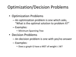
Decision Problems. Optimization problems : minimum, maximum, smallest, largest. Traveling salesman, Clique, Vertex-Cover, Independent Set, Knapsack. Satisfaction (SAT) problems :. CNF, Constraint-SAT, Hamiltonian Circuit, Circuit-SAT.

E N D
Decision Problems Optimization problems: minimum, maximum, smallest, largest Traveling salesman, Clique, Vertex-Cover, Independent Set, Knapsack Satisfaction (SAT) problems: CNF, Constraint-SAT, Hamiltonian Circuit, Circuit-SAT • Only optimization problems use theminimum, maximum, smallest, largest value: • To formulate the decision problem • As input parameter for Phase II of the non deterministic algorithms
Computing an Reduce and Conquer: Derek Drake’s: compute(a, n) { if (n=0) then return 1 m floor(n/2) s compute(a,m) if ( n is even) then return s * s if ( n is odd) then return a * s * s } Divide and Conquer: compute(a, n) { if (n=0) then return 1 m floor(n/2) return compute(a,m) × compute(a, n – m) } Brute Force: compute(a, n) { ans 1 for i 1 to n do ans ans * a return ans } Complexity: O(n) T(n) = 2T(n/2) +1 T(1) = 1 Complexity: O(n) T(n) = T(n/2) +3 T(1) = 1 Complexity: O(log2n)
Solving Recurrence Relations T(n) = 4T(n/2) + n T(1) = 1 T(n) = 4T(n/2) + n2 T(1) = 1 4k+ kn2 with n = 2k 4k+ 2k-1n + … + 2n + n with n = 2k O(n2 log2n) O(n2 )
Merge Sort is Stable • We split A into two parts B (first half) and C (first half) • Sort B and C separately • When merging B and C, we compare elements in B against elements in C, if tides occur, we insert element of B back into A first and then elements in B
Quicksort • An element of the array is chosen. We call it the pivot element. • The array is rearranged such that - all the elements smaller than the pivot are moved before it - all the elements larger than the pivot are moved after it • Then Quicksort is called recursively for these two parts.
Quicksort - Algorithm Quicksort (A[L..R]) if L < R then pivot = Partition( A[L..R]) Quicksort (A[1..L-1]) Quicksort (A[L+1...R)
Partition Algorithm Partition (A[L..R]) p A[L]; i L; j R + 1 while (i < j) do { repeat i i + 1 until A[i] ≥ p repeatj j - 1untilA[j] ≤ p if (i < j) then swap(A[i], A[j]) } swap(A[j],A[L]) return j
Example A [3 8 7 1 5 2 6 4]
Complexity Analysis • Best Case: every partition splits half of the array • Worst Case: one array is empty; one has all elements • Average case: O(n log2n) O(n2 ) O(n log2n)
Binary Search BinarySearch(A[1..n], el) Input: A[1..n] sorted in ascending order Output: The position i such that A[i] = el or -1 if el is not in A[1..n]