Mean and Standard Deviation of an 8-Sided Die

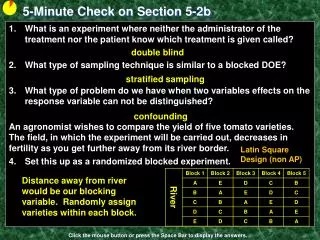
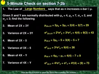
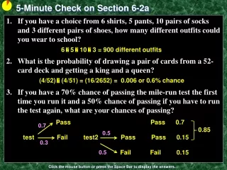
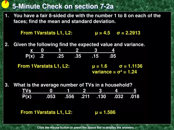
1. 5-Minute Check on section 7-2a You have a fair 8-sided die with the number 1 to 8 on each of the faces; find the mean and standard deviation. Given the following find the expected value and variance.x 0 1 2 3 4 P(x) .2 .25 .35 .15 .05 What is the average number of TVs in a household?TVs 0 1 2 3 4 5 P(x) .053 .556 .211 .130 .032 .018 From 1Varstats L1, L2: μ = 4.5 σ = 2.2913 From 1Varstats L1, L2: μ = 1.6 σ = 1.1136 variance = σ² = 1.24 From 1Varstats L1, L2: μ = 1.586 Click the mouse button or press the Space Bar to display the answers.

2. Lesson 7 – 2b Means and Variancesof Random Variables

3. Knowledge Objectives • Define what is meant by the mean of a random variable • Explain what is meant by a probability distribution • Explain what is meant by a uniform distribution • Discuss the shape of a linear combination of independent Normal random variables

4. Construction Objectives • Calculate the mean of a discrete random variable. • Calculate the variance and standard deviation of a discrete random variable. • Explain, and illustrate with an example, what is meant by the law of large numbers. • Explain what is meant by the law of small numbers. • Given µx and µy, calculate µa+bx, and µx+y. • Given x and y, calculate 2a+bx, and 2x+y (where x and y are independent). • Explain how standard deviations are calculated when combining random variables.

5. Vocabulary • Mean – balance point of the probability histogram or density curve. Symbol: μx • Standard Deviation – square root of the variance. Symbol: x • Variance – is the average squared deviation of the values of the variable from their mean. Symbol: σ²x

6. Law of Large Numbers • Sample mean, x, approaches population mean, μ, as sample size increases

7. Law of Small Numbers • People incorrectly believe that the long-term random behavior seen should also be seen in the short-term • We don’t expect to see long runs in the short-term because of this misperception • Intuition does not do a good job of distinguishing random behavior from systematic influences

8. Probability Laws • Law of Large Numbers – True • Sample mean, x, approaches population mean, μ, as sample size increases • Law of Small Numbers – False • Random behavior in short term does not mimic long-term behavior • Law of Averages – Bad Statistics • eventually everything evens out

9. Rules for Means • Means follow the rules for linear combinations (from Algebra) • When you linearly combine two or more (rules give only the 2 case example) random variables, you combine their means in the same manner

10. Rules for Variances • Adding a number to a random variable does not change its variance • Multiply a random variable by a number changes the variance by the square of that number • When you combine random variables, you always add the variances

11. Rules for Standard Deviations • Follow the rules for variances and then take the square root to find the standard deviation • In general standard deviations do not add • Note: independence is required for the calculations of combined variances, but not for means • Methods for combining non-independent variables’ variances involve covariance terms and are not part of this course

12. Example 1 Scores on a Math test have a distribution with μ = 519 and σ = 115. Scores on an English test have a distribution with μ = 507 and σ = 111. If we combine the scoresa) what is the combined mean b) what is the combined standard deviation? μM + μE = 519 + 507 = 1016 Scores are not independent so the following is not correct! σ²M+E = σ²M + σ²E = 115² + 111² = 25546 σM+E = 25546 = 159.83

13. Example 2 Suppose you earn $12/hour tutoring but spend $8/hour on dance lessons. You save the difference between what you earn and the cost of your lessons. The number of hours you spend on each activity is independent. Find your expected weekly savings and the standard deviation of your weekly savings.

14. Example 2 cont Expect value for Dancing, μX, is 0(0.4) + 1(0.3) + 2(0.3) = 0.9 Variance: ∑ [P(x) ∙ x2] – μx2 = (.4(0) + .3(1) + .3(4) ) – 0.9²) = 1.5 – 0.81 = 0.69 St Dev = 0.8307

15. Example 2 cont Expect value for Tutoring, μY, is 1(0.3) + 2(0.3) + 3(0.2) + 4(0.2) = 2.3 Variance: ∑ [x2 ∙ P(x)] – μx2 = (.3(1) + .3(4) + .2(9) + .2(16) ) – 2.3²) = 6.5 – 5.29 = 1.21 St Dev = 1.1

16. Example 2 cont Expected value for Weekly Savings, μ12Y-8X, is 12 μY - 8 μX = 12 (2.3) – 8 (0.9) = 27.6 – 7.2 = $20.4 Variance of Weekly Savings, σ²12Y-8X, is σ²12Y + σ²8X = 12²(1.21) + 8²(0.69) = 174.24 + 44.16 = 218.4 so standard deviation = $14.79

17. Combining Normal Random Variables • Any linear combination of independent Normal random variables is also Normally distributed • For example: If X and Y are independent Normally distributed random variables and a and b are any fixed numbers, then aX + bY is also Normally distributed • Mean and standard deviations can be found by using the rules from previous slides

18. Example 3 Tom’s score for a round of golf has a N(110,10) distribution and George’s score for a round of golf has a N(100,8) distribution. If they play independently, what is the probability that Tom will have a better (lower) score than George? Let X be Tom’s score and Y be George’s score μX-Y = μX - μY = 110 – 100 = 10 σ²X-Y = σ²X + σ²Y = 10² + 8² = 164 ≈ (12.8)² so X – Y is a N(10,12.8) P(X-Y<0) = P(z < Z) with Z = (0 – 10) / 12.8 = -0.78

19. Example 3 cont We could have used our calculator, ncdf(-E99,0,10,12.8), or Table A to get the probabilities illustrated in the graph below

20. Summary and Homework • Summary • Expected value is the mean ∑ [x ∙P(x)] • Variance is ∑[x2 ∙ P(x)] – μ2x • Standard Deviation is variance • Homework • pg 491; 7.32, 7.34 • pg 499; 7.37 - 7.40