Download
1 / 63
630 likes | 653 Views
Chapter 4 Risky Decisions. Arrow-Debreu general equilibrium, welfare theorem, representative agent. Radner economies real/nominal assets, market span, risk-neutral prob., representative good. von Neumann Morgenstern measures of risk aversion, HARA class. von Neumann Morgenstern

E N D
Arrow-Debreu general equilibrium, welfare theorem, representative agent Radner economies real/nominal assets, market span, risk-neutral prob., representative good von Neumann Morgenstern measures of risk aversion, HARA class von Neumann Morgenstern measures of risk aversion, HARA class Finance economy SDF, CCAPM, term structure Data and the Puzzles Empirical resolutions Theoretical resolutions
A very special ingredient: probabilities • By defining commodities as being contingent on the state of the world, we do in principle cover decisions involving risk already. • But risk has a special, additional structure which other situations do not have: probabilities. • We have not explicitly made use of probabilities so far. • The probabilities do affect preferences over contingent commodities, but so far we have not made this connection explicit. • The theory of decisions under risk exploits this particular structure in order to get more concrete predictions about behavior of decision-makers.
A hypothetical gamble • Suppose someone offers you this gamble: • "I have a fair coin here. I'll flip it, and if it's tail I pay you $1 and the gamble is over. If it's head, I'll flip again. If it's tail then, I pay you $2, if not I'll flip again. With every round, I double the amount I will pay to you if it's tail." • Sounds like a good deal. After all, you can't loose. So here's the question: • How much are you willing to pay to take this gamble?
The expected value of the gamble • The gamble is risky because the payoff is random. So, according to intuition, this risk should be taken into account, meaning, I will pay less than the expected payoff of the gamble. • So, if the expected payoff is X, I should be willing to pay at most X, possibly minus some risk premium. (We will discuss risk premia in detail later.) • BUT, the expected payoff of this gamble is INFINITE!
Infinite expected value • With probability 1/2 you get $1. • With probability 1/4 you get $2. • With probability 1/8 you get $4. • etc. • The expected payoff is the sum of these payoffs, weighted with their probabilities, so
probability $ An infinitely valuable gamble? • I should pay everything I own and more to purchase the right to take this gamble! • Yet, in practice, noone is prepared to pay such a high price. • Why? • Even though the expected payoff is infinite, the distribution of payoffs is not attractive… • With 93% probability we get $8 or less, with 99% probability we get $64 or less.
What should we do? • How can we decide in a rational fashion about such gambles (or investments)? • Bernoulli suggests that large gains should be weighted less. He suggests to use the natural logarithm. [Cremer, another great mathematician of the time, suggests the square root.] • Bernoulli would have paid at most eln(2) = $2 to participate in this gamble.
Lotteries • A risky payoff is completely described by a list of the possible payoffs and the probabilities associated with it. • We call such a risky payoff a lottery, but we could just as well call it a random variable. lottery L := [x1,p1 ; … ; xS,pS ]. • A non-risky payoff is a degenerate lottery [x,1].
Ordinal utility function • We assume that agents have preferences over lotteries. • Let L be the set of all lotteries. A preference relation is defined over elements of L. As before, ~ represents indifference (now between lotteries). • As before, we can represent these preferences with an ordinal utility function V. • Let L,L' є L be two lotteries, then V(L) < V(L') iff L L'.
Defn. risk aversion • The expected payoff of the lottery L = [x1,p1 ; … ; xS,pS ] is åspsxs =: E{L}. • We say that the agent is risk averse if V(L) < V([E{L},1]) (if L is not degenerate). • In words, the agent strictly prefers the average payoff of the lottery for sure as opposed to the risky lottery. • This means that the agent is willing to forego some payoff on average in exchange for not being exposed to the risk of the lottery.
Certainty equivalent • Consider some lottery L є L. If [x,1] ~ L then we call x the certainty equivalent of L. • Equivalently, V([x,1]) = V(L). • We denote x with CE(L). • CE(L) is the risk-free payoff that is equivalent to the risky payoff contained in lottery L.
Risk premium • An alternative way to define risk aversion is to require CE(L) < E{L} (if L is not degenerate). • We call the difference, E{L} – CE(L) =: RP(L) the risk premium. • It is the maximum premium the agent is willing to pay for an insurance that shields him from the risk contained in L.
The utility function V • In order to be able to draw indifference curves we will restrict attention to lotteries with only two possible outcomes, [x1,p1;x2,p2]. • Furthermore, we will also fix the probabilities (p1,p2), so that a lottery is fully described simply by the two payoffs (x1,x2). So a lottery is just a point in the plane. • From the ordinal utility function V we define a new function V that takes only the payoffs as an argument, V(x1,x2) = V([x1,p1;x2,p2]). • V is very much like a utility function over two goods that we have used in chapter 2. This makes it amenable to graphical analysis.
x2 45° x1 Indifference curves Any point in this plane is a particular lottery. Where is the set of risk-free lotteries? If x1=x2, then the lottery contains no risk.
x2 z 45° x1 z Indifference curves Where is the set of lotteries with expected prize E{L}=z? p It's a straight line, and the slope is given by the relative probabilities of the two states.
x2 z 45° x1 z Suppose the agent is risk averse. Where is the set of lotteries which are indifferent to (z,z)? Indifference curves ??? p That's not right! Note that there are risky lotteries with smaller expected prize and which are preferred.
x2 z 45° x1 z Indifference curves So the indifference curve must be tangent to the iso-expected-prize line. This is a direct implication of risk-aversion alone. p
x2 z 45° x1 z Indifference curves But risk-aversion does not imply convexity. p This indifference curve is also compatibe with risk-aversion.
x2 z 45° x1 z Indifference curves The tangency implies that the gradient of V at the point (z,z) is collinear to p. V(z,z) p Formally, V(z,z) = lp, for some l>0.
What we are after: an expected utility representation • The ordinal utility function V is a cumbersome object because its domain is a large set, L, the set of all lotteries. • A utility function on prizes (and the expected value of such a utility function, given a lottery), would be much easier to work with. • So we look for a representation of the form V([x1,p1; …; xS,pS]) = åspsv(xs).
x y p 1-p ~ p 1-p y x NM axioms: state independence • Von Neumann and Morgenstern have presented a model that allows the use of an expected utility under some conditions. • The first assumption is state independence. • It means that the names of the states have no particular meaning and are interchangeable. • Note that this rules out the case where you have different preferences over wealth if it rains or if the weather's bright.
p11 p1 p11 x1 x1 L1 p1 x2 p1 p12 p12 x2 ~ p21 x3 p2 p21 x3 p2 p2 p22 L2 p22 x4 x4 NM axioms: consequentialism • Consider a lottery whose prices are further lotteries, L = [L1,p1;L2,p2]. This is a compound lottery. • The axiom requires that agents are only interested in the distribution of the resulting prize, but not in the process of gambling itself.
L1 L2 p 1-p p 1-p x x L1L2 NM axioms: irrelevance of common alternatives • This axiom says that the ranking of two lotteries should depenend only on those outcomes where they differ. • If L1 is better than L2, and we compound each of these lotteries with some third common outcome x, then it should be true that [L1,p;x,1-p] is still better than [L2,p;x,1-p]. The common alternative x should not matter.
v(x) Consider a fifty-fifty lottery with two prizes… v(x1) E{v(x)} v(x0) x0 x1 x Risk-aversion and concavity • Von Neumann and Morgenstern prove that with these assumptions, one can represent a utility over lotteries V as an expected utility v. • The shape of the von Neumann Morgenstern (NM) utility function contains a lot of information. • How does the NM utility function of a risk-neutral agent look like? E{x}
v(x) v(x1) E{v(x)} v(x0) x0 x1 x v-1(E{v(x)}) Risk-aversion and concavity • Risk-aversion means that the certainty equivalent is smaller than the expected prize. • We conclude that a risk-averse NM utility function must be concave. E{x}
An insurance problem • Consider an insurance problem: • d amount of damage, • p probability of damage, • m insurance premium for full coverage, • c amount of coverage. The FOC of this problem is
An insurance problem • Full coverage (c=1) implies Full coverage is optimal only if the premium is statistically fair. • Suppose the premium is not fair. Let m = (1+m)pd, and m>0 be the insurance company's markup. Then,
An insurance problem • If the insurance premium is not fair, it is optimal not to fully insure. • In fact, if the premium is large enough (m0), no coverage is optimal. • The FOC, with m substituted by (1+m)pd, is • We extract m0 by setting c=0, and then solve for m0
An insurance problem • If m=(1+m0)pd, the agent is just indiff between insuring and carrying the whole risk. • Thus, w-(1+m0)pd is the certainty equivalent. • It is clear that m0 vanishes as the risk becomes smaller, pd 0. • But the relative speed of convergence is not so clear: how fast does m0 vanish compared topd?
Note that this part is just the second derivative of v… …and this part converges to the first derivative. Absolute risk aversion For symmetric risks (p=1/2) we thus get This is the celebrated coefficient of absolute risk aversion, discovered by Pratt and by Arrow. We see here that it is a measure for the size of the risk premium for an infinitesimal risk.
CARA, IARA, DARA • Consider some utility function and its associated absolute risk aversion as a function of wealth, A(w). • We say that absol risk aversion is decreasing (DARA) if A'(w)<0; it is constant (CARA) if A'(w)=0; it is increasing (IARA) if A'(w)>0. • Consider then two people, both with the same utility function, but one is very poor, the other very rich. • Suppose also that both agents are subject to the same risk of losing, say, $10. • How of the two is more willing to insure against this risk?
CARA, IARA, DARA • It seems reasonable to assume that the rich person is not willing to insure, because he will not notice the difference of $10. • The very poor person, on the other hand, may be very eager to insure, because $10 amounts to a substantial part of his wealth. • If this is the case, then utility is DARA. • IARA would imply that the rich person buys insurance against this risk, but the poor does not, which seems not plausible.
Relative risk aversion • We have considered additive risks so far: lose $10 with some probability, or experience a damage d with probability p. • But some risks are multiplicative (risking 10% of your wealth). This is particularly true in financial markets: if you invest 20% of your wealth in shares, then you are exposed to a multiplicative risk. • Relative risk aversion rather than absolute risk aversion is the correct measure to estimate the willingness to insure against infinitesimal multiplicative risks.
Relative risk aversion R(w) := wA(w). • Consider the rich and poor people of before again, but now suppose they are both subject to a 50% risk of losing 10% of their wealth. • Which of the two is willing to pay a larger share of his wealth to insure against this risk? • This seems unclear a priori. If both have the same willingness to pay (as a percentage of their wealth), the utility function exhibits constant relative risk aversion (CRRA). • The other possibilities are IRRA and DRRA.
Prudence • The measures of risk aversion inform us about the willingness to insure … • … but they do not inform us about the comparative statics. • How does the behavior of an agent change when we marginally increase his exposure to risk? • An old hypothesis (going back at least to J.M.Keynes) is that people should save more now when they face greater uncertainty in the future. • The idea is called precautionary saving and has intuitive appeal.
Prudence • But it does not directly follow from risk aversion alone. • In fact, it involves the third derivative of the utility function. • Kimball (1990) defines absolute prudence as P(w) := –v'''(w)/v''(w). • He shows that agents have a precautionary saving motive if any only if they are prudent. • This finding will be important later on when we do comparative statics of interest rates. • Prudence seems uncontroversial, because it is weaker than DARA.
Uncontroversial properties • Monotonicity seems uncontroversial. After all, most people prefer more wealth to less. • Risk aversion is only slightly more controversial. Of course, there may be some risk seekers. But most people shun risks. • DARA also seems reasonable. • And since DARA implies prudence, we should also expect people to be prudent.
Animal experiments • Kagel et al. (1995) have performed interesting experiments with animals. • Payoff is food. • Very good control over "wealth" (nutritional level) of animals. • They find evidence for risk aversion and DARA. • In fact, they find some weak evidence for a utility function of the form (x-s)1-g/(1-g), where x is consumption and s>0 can be interpreted as subsistence level (see chapter 6.3 of their book). • This utility function exhibits DRRA as well.
Empirical estimates • Friend and Blume (1975): study U.S. household survey data in an attempt to recover the underlying preferences. Evidence for DARA and almost CRRA, with R 2. • Tenorio and Battalio (2003): TV game show in which large amounts of money are at stake. Estimate rel risk aversion between 0.6 and 1.5. • Abdulkadri and Langenmeier (2000): farm household consumption data. They find significantly greater risk aversion. • Van Praag and Booji (2003): large survey done by a dutch newspaper. They find that rel risk aversion is close to log-normally distributed, with a mean of 3.78.
Introspection • In order to get a feeling for what different levels of risk aversion actually mean, it may be helpful to find out what your own personal coefficient of risk aversion is. • You can do that by working through Box 4.6 of the book, or by using the electronic equivalent available from the website. LAUNCH
Evolutionary stability • A completely different take on the problem is provided by evolutionary finance. • Natural selection, so the argument, favors agents with relative risk aversion close to unity. • The reason is that such agents maximize the growth rate of their wealth, and thus eventually dominate the market. • Thus, either you maximize ln(y), or you are eventually marginalized. • With this line of argument, experiments, empirics or introspection are not needed, because in the long run the market is necessarily dominated by lof utility functions. • Literature: Hakansson (1971), Blume and Easly (1992), Sinn and Weichenrieder (1993), Sinn (2002).
Usual utility functions One finds only a handful of specifications in the literature. A, R, and P denote absolute risk aversion, relative risk aversion, and prudence. a and b will be explained later.
The HARA class • All the functions of the previous tables belong to the hyperbolic absolute risk aversion, or HARA, class. (An alternative name is linear risk tolerance, or LRT.) • Let absolute risk tolerance be defined as the reciprocal of absolute risk aversion, T := 1/A. • u is HARA if T is an affine function, T(y) = a + by. • The slope b is is sometimes also called cautiousness.