Download

1 / 60
600 likes | 619 Views
Multimedia and Text Indexing. Midterm. Monday, March 19, 2018 in class Closed Books and notes One cheat sheet: 8.5" by 11" sheet of notes (both sides) Topics Spatial Temporal Spatio -temporal Time Series All papers and lecture notes on these topics. Multimedia Data Management.

E N D
Midterm • Monday, March 19, 2018 in class • Closed Books and notes • One cheat sheet: 8.5" by 11" sheet of notes (both sides) • Topics • Spatial • Temporal • Spatio-temporal • Time Series • All papers and lecture notes on these topics
Multimedia Data Management • The need to query and analyze vast amounts of multimedia data (i.e., images, sound tracks, video tracks) has increased in the recent years. • Joint Research from Database Management, Computer Vision, Signal Processing and Pattern Recognition aims to solve problems related to multimedia data management.
Multimedia Data • There are four major types of multimedia data: images, video sequences, sound tracks, and text. • From the above, the easiest type to manage is text, since we can order, index, and search text using string management techniques, etc. • Management of simple sounds is also possible by representing audio as signal sequences over different channels. • Image retrieval has received a lot of attention in the last decade (CV and DBs). The main techniques can be extended and applied also for video retrieval.
Content-based Image Retrieval • Images were traditionally managed by first annotating their contents and then using text-retrieval techniques to index them. • However, with the increase of information in digital image format some drawbacks of this technique were revealed: • Manual annotation requires vast amount of labor • Different people may perceive differently the contents of an image; thus no objective keywords for search are defined • A new research field was born in the 90’s: Content-based Image Retrieval aims at indexing and retrieving images based on their visual contents.
Feature Extraction • The basis of Content-based Image Retrieval is to extract and index some visual features of the images. • There are general features (e.g., color, texture, shape, etc.) and domain-specific features (e.g., objects contained in the image). • Domain-specific feature extraction can vary with the application domain and is based on pattern recognition • On the other hand, general features can be used independently from the image domain.
Color Features • To represent the color of an image compactly, a color histogram is used. Colors are partitioned to k groups according to their similarity and the percentage of each group in the image is measured. • Images are transformed to k-dimensional points and a distance metric (e.g., Euclidean distance) is used to measure the similarity between them. k-dimensional space k-bins
Using Transformations to Reduce Dimensionality • In many cases the embedded dimensionality of a search problem is much lower than the actual dimensionality • Some methods apply transformations on the data and approximate them with low-dimensional vectors • The aim is to reduce dimensionality and at the same time maintain the data characteristics • If d(a,b) is the distance between two objects a, b in real (high-dimensional) and d’(a’,b’) is their distance in the transformed low-dimensional space, we want d’(a’,b’)d(a,b). d’(a’,b’) d(a,b)
MultimediaIndexing Every indexing model must follow a retrieval semantics. The multimedia indexing model must support the similarity queries. Two types similarity queries: • range queriesreturn documents similar more than a given threshold • k nearest neighbour queriesreturn the first k most similar documents
MetricIndexing Feature vectors are indexed according to distances between each other. As a dissimilarity measure, a distance function d(Oi,Oj)is specified such that the metric axioms are satisfied: d(Oi,Oi)= 0 reflexivity d(Oi,Oj) > 0 positivity d(Oi,Oj) = d(Oj,Oi) symmetry d(Oi,Ok) + d(Ok,Oj)≥d(Oi,Oj) triangular inequality Metric structures: Main memory structures: cover-tree, vp-tree, mvp-tree Disk-based structures: M-tree, Slim-tree
The M-tree • Inherently dynamic structure • Disk-oriented (fixed-size nodes) • Built in a bottom-up fashion • Inspired by R-trees and B-trees • All data in leaf nodes • Internal nodes: pointers to subtrees and additional information http://www.nmis.isti.cnr.it/amato/similarity-search-book/slides/
M-tree: Internal Node • Internal node consists of an entry for each subtree • Each entry consists of: • Pivot: p • Covering radius of the sub-tree: rc • Distance from p to parent pivot pp: d(p,pp) • Pointer to sub-tree: ptr • All objects in subtree ptr are within the distance rc from p.
M-tree: Leaf Node • leaf node contains data entries • each entry consists of pairs: • object (its identifier): o • distance between o and its parent pivot: d(o,op)
o9 o8 o6 o4 o11 o10 o5 o7 o1 o2 o3 1.2 1.6 0.0 1.0 1.3 1.4 2.9 0.0 0.0 0.0 0.0 o10 o7 o7 o4 o1 o1 o2 o2 o10 2.9 4.5 1.6 6.9 1.3 1.2 1.4 3.8 0.0 0.0 3.3 5.3 -.- -.- o2 M-tree: Example o5 o11 o3 o8 o1 Covering radius o6 o4 o9 Distance to parent Distance to parent
M-tree: Insert • Insert a new object oN: • recursively descend the tree to locate the most suitable leaf for oN • in each step enter the subtree with pivot p for which: • no enlargement of radius rc needed, i.e., d(oN,p) ≤ rc • in case of ties, choose one with p nearest to oN • minimize the enlargement of rc
M-tree: Insert (cont.) • when reaching leaf node N then: • if N is not full then store oN in N • else Split(N,oN).
M-tree: Split Split(N,oN): • Let S be the set containing all entries of N and oN • Select pivots p1and p2 from S • Partition S to S1 and S2 according to p1and p2 • Store S1in N and S2in a new allocated node N’ • If N is root • Allocate a new root and store entries for p1, p2 there • else (let Np and pp be the parent node and parent pivot of N) • Replace entry pp with p1 • If Np is full, then Split(Np,p2) • else store p2 in node Np
M-tree: Pivot Selection • Several pivots selection policies • RANDOM – select pivots p1, p2 randomly • m_RAD – select p1, p2 with minimum (r1c + r2c) • mM_RAD – select p1, p2 with minimum max(r1c, r2c) • M_LB_DIST – let p1 = pp and p2 = oi | maxi { d(oi,pp) } • Uses the pre-computed distances only • Two versions (for most of the policies): • Confirmed – reuse the original pivot pp and select only one • Unconfirmed – select two pivots (notation: RANDOM_2) • In the following, the mM_RAD_2 policy is used.
Unbalanced Generalized hyperplane Balanced Larger covering radii p2 p1 M-tree: Split Policy • Partition S to S1 and S2 according to p1and p2 p2 p1
q q M-tree: Range Search Given R(q,r): • Traverse the tree in a depth-first manner • In an internal node, for each entry p,rc,d(p,pp),ptr • Prune the subtree if |d(q,pp) – d(p,pp)| – rc > r • Application of the pivot-pivot constraint r pp pp p rc r p rc
r rc p q M-tree: Range Search (cont.) • If not discarded, compute d(q,p) and • Prune the subtree if d(q,p) – rc > r • Application of the range-pivot constraint • All non-pruned entries are searched recursively.
M-tree: Range Search in Leaf Nodes • In a leaf node, for each entry o,d(o,op) • Ignore entry if |d(q,op) – d(o,op)| > r • else compute d(q,o)and check d(q,o) ≤ r • Application of the object-pivot constraint
M-tree: k-NN Search Given k-NN(q): • Based on a priority queue and the pruning mechanisms applied in the range search. • Priority queue: • Stores pointers to sub-trees where qualifying objects can be found. • Considering an entry E=p,rc,d(p,pp),ptr, the pair ptr,dmin(E) is stored. • dmin(E)=max { d(p,q) – rc, 0 } • Range pruning: instead of fixed radius r, use the distance to the k-th current nearest neighbor.
Text Retrieval (Information retrieval) • Given a database of documents, find documents containing “data”, “retrieval” • Applications: • Web • law + patent offices • digital libraries • information filtering
Problem - Motivation • Types of queries: • boolean (‘data’ AND ‘retrieval’ AND NOT ...) • additional features (‘data’ ADJACENT ‘retrieval’) • keyword queries (‘data’, ‘retrieval’) • How to search a large collection of documents?
Text – Inverted Files Q: space overhead? A: mainly, the postings lists
how to organize dictionary? stemming – Y/N? Keep only the root of each word ex. inverted, inversion invert insertions? Text – Inverted Files
how to organize dictionary? B-tree, hashing, TRIEs, PATRICIA trees, ... stemming – Y/N? insertions? Text – Inverted Files
Text – Inverted Files • postings list – more Zipf distr.: eg., rank-frequency plot of ‘Bible’ log(freq) freq ~ 1/rank / ln(1.78V) log(rank)
Text – Inverted Files • postings lists • Cutting+Pedersen • (keep first 4 in B-tree leaves) • how to allocate space: [Faloutsos+92] • geometric progression • compression (Elias codes) [Zobel+] – down to 2% overhead! • Conclusions: needs space overhead (2%-300%), but it is the fastest
Text - Detailed outline • Text databases • problem • inversion • signature files (a.k.a. Bloom Filters) • Vector model and clustering • information filtering and LSI
Vector Space Model and Clustering • Keyword (free-text) queries (vs Boolean) • each document: -> vector (HOW?) • each query: -> vector • search for ‘similar’ vectors
Vector Space Model and Clustering • main idea: each document is a vector of size d: d is the number of different terms in the database document zoo aaron data ‘indexing’ ...data... d (= vocabulary size)
Document Vectors • Documents are represented as “bags of words” OR as vectors. • A vector is like an array of floating points • Has direction and magnitude • Each vector holds a place for every term in the collection • Therefore, most vectors are sparse
Document VectorsOne location for each word. A B C D E F G H I nova galaxy heat h’wood film role diet fur 10 5 3 5 10 10 8 7 9 10 5 10 10 9 10 5 7 9 6 10 2 8 7 5 1 3 “Nova” occurs 10 times in text A “Galaxy” occurs 5 times in text A “Heat” occurs 3 times in text A (Blank means 0 occurrences.)
Document VectorsOne location for each word. A B C D E F G H I nova galaxy heat h’wood film role diet fur 10 5 3 5 10 10 8 7 9 10 5 10 10 9 10 5 7 9 6 10 2 8 7 5 1 3 “Hollywood” occurs 7 times in text I “Film” occurs 5 times in text I “Diet” occurs 1 time in text I “Fur” occurs 3 times in text I
Document Vectors nova galaxy heat h’wood film role diet fur 10 5 3 5 10 10 8 7 9 10 5 10 10 9 10 5 7 9 6 10 2 8 7 5 1 3 Document ids A B C D E F G H I
We Can Plot the Vectors Star Doc about movie stars Doc about astronomy Doc about mammal behavior Diet
Assigning Weights to Terms • Binary Weights • Raw term frequency • tf x idf • Recall the Zipf distribution • Want to weight terms highly if they are • frequent in relevant documents … BUT • infrequent in the collection as a whole
Binary Weights • Only the presence (1) or absence (0) of a term is included in the vector
Raw Term Weights • The frequency of occurrence for the term in each document is included in the vector
Assigning Weights • tf x idf measure: • term frequency (tf) • inverse document frequency (idf) -- a way to deal with the problems of the Zipf distribution • Goal: assign a tf * idf weight to each term in each document
Inverse Document Frequency • IDF provides high values for rare words and low values for common words For a collection of 10000 documents
Similarity Measures for document vectors (seen as sets) Simple matching (coordination level match) Dice’s Coefficient Jaccard’s Coefficient Cosine Coefficient Overlap Coefficient
tf x idf normalization • Normalize the term weights (so longer documents are not unfairly given more weight) • normalize usually means force all values to fall within a certain range, usually between 0 and 1, inclusive.
Vector space similarity(use the weights to compare the documents)
Computing Similarity Scores 1.0 0.8 0.6 0.4 0.2 0.2 0.4 0.6 0.8 1.0
Vector Space with Term Weights and Cosine Matching Di=(di1,wdi1;di2, wdi2;…;dit, wdit) Q =(qi1,wqi1;qi2, wqi2;…;qit, wqit) Term B 1.0 Q = (0.4,0.8) D1=(0.8,0.3) D2=(0.2,0.7) Q D2 0.8 0.6 0.4 D1 0.2 0 0.2 0.4 0.6 0.8 1.0 Term A