Download
1 / 72
720 likes | 729 Views
Probabilistic Object Recognition and Localization. Bernt Schiele, Alex Pentland, ICCV ‘99 Presenter: Matt Grimes. What they did. Chose a set of local image descriptors whose outputs are robust to object orientation and lighting. Examples:. First-derivative magnitude:. Laplacian.

E N D
Probabilistic Object Recognition and Localization Bernt Schiele, Alex Pentland, ICCV ‘99 Presenter: Matt Grimes
What they did • Chose a set of local image descriptors whose outputs are robust to object orientation and lighting. • Examples: First-derivative magnitude: Laplacian
What they did • Learn a PDF for the outputs of these descriptors given an image of the object: Object orientation, lighting, etc. Vector of descriptor outputs A particular object
What they did • Learn a PDF for the outputs of these descriptors given an image of the object: Vector of descriptor outputs A particular object
What they did • Use Bayes’ rule to obtain the posterior… • …which is the probability of an image containing an object, given local image measurements M. • (Not quite this clean)
History of image-based object recognition Two major genres: • Histogram-based approaches. • Comparison of local image features.
Histogramming approaches • Object recognition by color histograms (Swain & Ballard, IJCV 1991) • Robust to changes in orientation, scale. • Brittle against lighting changes (dependency on color). • Many classes of objects not distinguishable by color distribution alone.
Histogramming approaches • Combat color-brittleness using (quasi-) invariants of color histograms: • Eigenvalues of matrices of moments of color histograms • Derivatives of logs of color channels • “Comprehensive color normalization”
Histogramming approaches • Comprehensive color normalization examples:
Histogramming approaches • Comprehensive color normalization examples:
Localized feature approaches • Approaches include: • Using image “interest-points” to index into a hashtable of known objects. • Comparing large vectors of local filter responses.
Geometric Hashing • An interest point detector finds the same points on an object in different images. Types of “interest points” include corners, T-junctions, sudden texture changes.
Geometric Hashing From Schmid, Mohr, Bauckhage, “Comparing and Evaluating Interest Points,” ICCV ‘98
Geometric Hashing From Schmid, Mohr, Bauckhage, “Comparing and Evaluating Interest Points,” ICCV ‘98
Geometric Hashing • Store points in an affine-transform-invariant representation. • Store all possible triplets of points as keys in a hashtable.
Geometric Hashing • For object recognition, find all triplets of interest points in an image, look for matches in the hashtable, accumulate votes for the correct object. Hashtable approaches support multiple object recognition within the same image.
Geometric hashing weaknesses • Dependent on the consistency of the interest point detector used. From Schmid, Mohr, Bauckhage, “Comparing and Evaluating Interest Points,” ICCV ‘98
Geometric hashing weaknesses • Shoddy repeatibility necessitates lots of points. • Lots of points, combined with noise, leads to lots of false positives.
Vectors of filter responses • Typically use vectors of oriented filters at fixed grid points, or at interest points. • Pros: • Very robust to noise. • Cons: • Fixed grid needs large representation, large grid is sensitive to occlusion. • If using an interest point detector instead, the detector must be consistent over a variety of scenes.
Also: eigenpictures • Calculate the eigenpictures of a set of images of objects to be recognized. • Pros: • Efficient representation of images by their eigenpicture coefficients. (Fast searches) • Cons: • Images must be pre-segmented. • Eigenpictures are not local (sensitive to occlusion). • Translation, image-plane rotation must be represented in the eigenpictures.
This paper: • Uses vectors of filter responses, with probabilistic object recognition. Learned from training images Using scene-invariant M Bayes’ rule
Wins of this paper • Uses hashtables for multiple object recognition. • Unlike geometric hashing, doesn’t depend on point correspondence betw. images. • Uses location-unspecific filter responses, not points. • Inherits robustness to noise of filter response methods.
Wins of this paper • Uses local filter responses. • Robust to occlusion compared to global methods (e.g. eigenpictures or filter grids.) • Probabilistic matching • Theoretically cleaner than voting. • Combined with local filter responses, allows for localization of detected objects.
Details of the PDF • What degrees of freedom are there in the “other” parameters? on: Object R: Rotation (3 DOF) T: Translation(3 DOF) S: Scene (occlusions, background) L: Lighting I: Imaging (noise, pixelation/blur)
P(M|on,R,T,S,L,I) • Way too many params to get a reliable estimate from even a large image library. • # of examples needed is exponential in the number of dimensions of the PDF. • Solution: choose measurements (M) that are invariant with respect to as many params as possible (except on).
Techniques for invariance • Imaging (noise:) see Schiele’s thesis. • Lighting: apply a “energy normalization technique” to the filter outputs. • Scene: probabilistic object recognition + local image measurements. • Gives best estimate using the visible portion of the object.
Techniques for invariance • Translation: • Tx, Ty (image-plane translation) are ignored for non-localizing recognition. • Tz is equivalent to scale. For known scales, compensate by scaling the filters’ regions of support.
Techniques for invariance • Fairly robust to unknown scale:
Techniques for invariance • Rotation: • Rz: rotation in the image plane. Filters invariant to image-plane rotation may be used. • Rx, Ry must remain in the PDF. Impossible to have viewpoint- invariant descriptors in the general case.
New PDF • 4 parameters. • Still a large amount of training examples needed, but feasible. • Example: algorithm has been successful after training with 108 images per object. (108 = 16 orientations * 6 scales)
Learning & representation of the PDF • Since the goal is discrimination, overgeneralization is scarier than overfitting. • They chose multidimensional histograms over parametric representations. • They mention that they could’ve used kernel function estimates.
Multidimensional Histograms • In their experiments, they use a 6-dimensional histogram. • X and Y derivative, at 3 different scales • …with 24 buckets per axis. • Theoretical max for # of cells: 246=1.9 x 10⁸ • Way too many cells to be meaningfully filled by even 512 x 512 (=262144 ) pixel images.
Multidimensional Histograms • Somehow, by exploiting dependencies betw. histogram axes, and applying a uniform prior bias, they get the number of calculated cells below 105. • Factor of 1000 reduction. • Anybody know how they do this?
(Single) object recognition • A single measurement vector mk is insufficient for recognition.
(Single) object recognition • A single measurement vector mk is insufficient for recognition.
(Single) object recognition • For k measurement vectors:
(Single) object recognition • Measurement regions covering 10~20% of an object are usually sufficient for discrimination.
Multiple object recognition • We can apply the single-object detector to many small regions in the image.
Multiple object recognition • The algorithm is now O(NKJ) • N = # of known objects • K = # of measurement vectors in each region • J = # of regions