Segmentation, area based

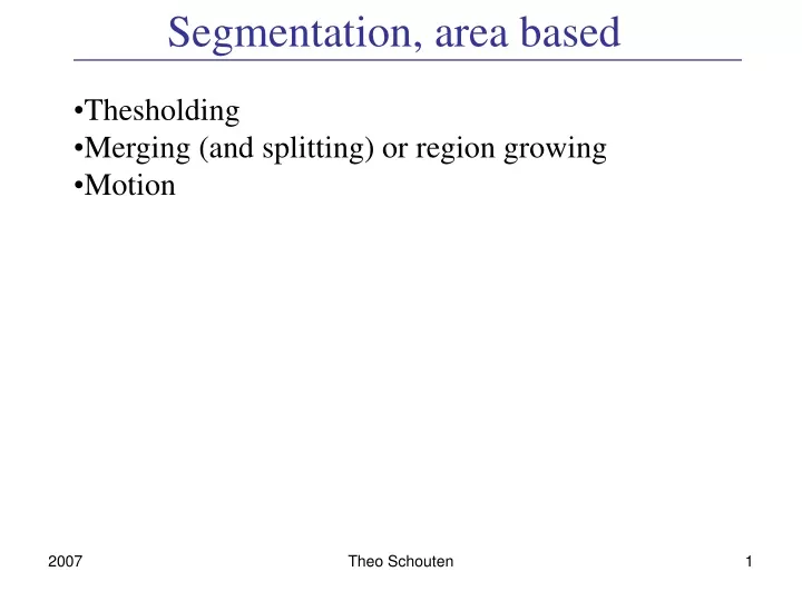
1. Segmentation, area based • Thesholding • Merging (and splitting) or region growing • Motion Theo Schouten

2. Thresholding Landsat image and histogram pixels with intensity < 18 (water pixels) pixels with intensity between 138 and 148 These are not yet segments! need also to make connected regions out of it. Theo Schouten

3. Finding thresholds There are many methods to automatically find the optimum (in some sense) threshold from a histrogram, Note that there will often be misclassified pixels, they have to be handled when forming the regions. Theo Schouten

4. per subimage • per subimage look to histogram: • 2 peaks: determine threshold • 1 peak: use neighoring or global threshold Pixels on the edge of objects have a gray value between that of the object and that of the background. Making a gray level histogram of only pixels having a large edge value yields a peak, which is a good choice for the threshold. Theo Schouten

5. further division Also, only the pixels with a small gradient can be taken or the pixels can be weighted with a factor 1/(1+G2). This results in sharper peaks and deeper valleys. One can also construct and analyze a 2-D histogram out of gray and edge values. Theo Schouten

6. Color • With color (in general a vector value) images we can get intensity histograms for each different component, and also combinations thereof (for example R,G,B or I,H,S or Y,I,Q by color). • The component with the best peak separation can then be chosen to yield the threshold for separating the object from the background. • This method can be extended to a recursive segmentation algorithm, by doing the following for each region: • - calculate the histograms for each of the vector components.- take the component with the best separation between two peaks and determine the threshold values to the left and to the right of the best peak. Divide the area into two parts (pixels inside and outside of that peak), according to those threshold values.- every sub-area can now have a noisy contour, improve to make neat connected regions.- repeat the previous steps for each sub-area, until no histogram has a protruding peak. Theo Schouten

7. other components In (a) this method does not lead to a good segmentation, in contrary to that of (b). Using R+G and R-G components in (a) would have led to a good segmentation. For (a) we can also use the 2-dimensional histogram directly to look for peaks. Of course this is more difficult than looking for peaks in a 1-D histogram. Theo Schouten

8. Split and merge The regions found using the previous methods are uniquely homogenous, resulting in a Boolean function H(R) with:   H( Rk ) = true    for all regions k  H( Ri Rj ) = false  for i    j combined regions For example  | f(x,y) - f(x',y')| < T  , the regions pass the peak test. Horowitz and Pavlides (1974) organize the image pixels into a (pyramid) grid structure. Every region (except for 1 pixel areas) can be split up into 4 regions. Four regions on the correct position can be joined again to make 1 region. They used this structure in the following split and merge join algorithm working for every function H(): - begin with all the regions on a satisfactory level in the pyramid.  - if there is a Rk with H(Rk) = false, then divide the Rk into four even parts.  - if for the 4 sub regions, lying on the correct position, the following holds H( Rk1  Rk2 Rk3   Rk4) = true, then join the 4 sub regions together to Rk.  - repeat the last two steps until there is nothing left to divide or join  - finally join the regions together that do not fit into the pyramid structure neatly. Theo Schouten

9. Region growing • Image showing defective welds • Selected “seed” points, pixels with a value of 255. • Result of region growing according certain criteria. • Boundaries of segmented defective welds. Theo Schouten

10. Best Merge First all the 4-connected pixels are joined into one region if they are exactly alike. Then the two 4-connected regions with the smallest error criterium for merging are combined together to 1 region. This is repeated until the error criterium is larger than a certain threshold. Choosing the “right” stopping value is a difficut problem. For the Landsat satellite image, the error criteria between two regions i and j was: Eij =  ( c (ci -   cj)2ck is the average value of the area k in band c Also other E’s could be used, e.g. taking the size of the regions to favour merging of small regions with large ones. Also the ’s of the regions could be taken into account. Theo Schouten

11. example Landsat 1 band, threshold 6 1 band, threshold 10 1 band, threshold 16 all bands, threshold 6 Theo Schouten

12. Watershed segmentation • 3 kinds of pixels: • pixels belonging to a local minimum • catchment bassin or watershed: pixels at which a drop of water would flow to that local minimum • divide of watershed lines: pixels at which water would flow to two mimima. Theo Schouten

13. Watershed 2D View the image in 3D: x,y and gray level Need “dam” construction to prevent too much merging of watersheds. Theo Schouten

14. example watershed Image of blobs and gradient image Watershed lines of gradient image superimposed on origina; Theo Schouten

15. using “markers” Adding “markers”: internal: belong to objects of interest external: associated with the background Theo Schouten

16. another example Theo Schouten

17. Motion, optical flow The "optical flow" method assigns a 2-dimensional speed vector to each pixel. This vector shows the direction and speed with which the portrayed pixel has moved. No specific knowledge about the portrayed scene is used. A time series of images is modeled as a function f(x,y,t), where it is assumed that f is "neat": the function is continuous and can be differentiated. Assume that during t the image moves over x and y:   f(x,y,t) = f(x+x, y+y, t+ t) At small x, y and t and because f is "neat" we can write the Taylor expansion of f: f(x+x, y+y, t+ t) = f(x,y,t) + f/x  x +  f/y  y + f/ t   t + e The expansion part must thus be 0, and after neglecting e (the higher order terms):  - f/t =  f/x  x/t + f/y  y/ t  =  f/x  u +  f/y  v   with  u= (u,v)  the speed vector  =   f . u       with f  the gradient of f The gradient for each pixel can be determined from each image, and f/ t from two consecutive images. The equation above restricts u for every pixel to ly on a line in the (u,v) space. Theo Schouten

18. Special reduncandy, Horn and Schunk Spatial redundancy" can be used to determine u because neighboring pixels often have almost the same speed. Horn and Schunck used this in the requirement that the derivative of the speed must be as small as possible. This leads to the minimization of the following cost or energy function (with a Lagrange multiplier):  E(x,y) = (fxu + fyv + ft )2 +   (ux2 + uy2 + vx2 + vy2 ) ( fx is f/x, etc.) Differentiate towards u (and the same for v) and equal it to 0:  2 (fxu + fyv + ft) fx + 2  ( 2u/x2 + 2u/ y2 ) = 0 The last term is the Laplacian 2u, which we approximate by:   u(x,y) - 0.25{ u(x,y+1)+u(x,y-1)+u(x+1,y)+u(x-1,y) } or in other words: 2u= u - uav Working this out further results in:  u = uav - fx  P/D  with P = fx uav + fy vav + ft v = vav - fy  P/D        D =   + fx2 + fy2 We solve these equations iteratively for u and v using the Gauss-Seidel method. Theo Schouten

19. examples This method only works well for areas with a strong texture (local deviations in intensity) because then there is a decent gradient.With small gradients the noise results in a relatively large error on the gradient, which continues to work on large errors on u. In fact the motion can only determined well in the direction of edges. Theo Schouten

20. Results by Miki Elad Row A gives the real optical flow from the synthetic series of images, row D gives the results of the Horn and Schunck algorithm. Rows B and C give the results of Miki Elad making use of the recursive approximated Kalman Filter algorithms. Theo Schouten

21. Focus of Expansion When we move in an environment with static objects, then the visual world, as projected on the retina, seems to slide by. For a given direction of the linear movement and given the direction in which to look, the world seems to come from one certain point in the retina, called the "focus of expansion" or FOE. If we take a perspective projection, such as a lens, from the origin looking in the positive Z direction with the image plane in z = 1, then : xi = x / z and  yi = y / z Let all the objects move linearly with a speed of: (x/t, y/t, z/t) = (u,v,w). In the image plane the movement of a point starting at (x0,y0,z0) becomes:              ( xi, yi ) = ( (x0 + ut) / (z0 + wt) , (y0 +vt ) / (z0 + wt) ) From this we can derive xi = m yi + c where m and c are constants, independent of t. This movement thus follows a straight line that comes from ( taking t = -) the point (u/w, v/w). This is independent of the position (x0,y0,z0) of the point, every point on an object seems to come from (u/w, v/w), this is the FOE. Theo Schouten

22. Correspondence problem The algorithms for this are often composed of two steps. First candidate match points are found in each image independently. To do this one must choose image points that somehow deviate strongly from its environment. To do this, Moravec first defined deviation values for each pixel:   var(x,y) =   {f(x,y) - f(x+k,y+l)}2 with (k,l) in (-a,-a)...(a,a) IntOp(x,y) = min s,t var(s,t)   with (s,t) in the environment of (x,y) The IntOp values having the local maximum and those larger than a certain threshold value are chosen as candidate match points. This threshold value can be adjusted locally to yield a good distribution of candidates over the image. Corners or sharp bends of object contours are also good interest points Theo Schouten

23. matching Barnard and Thompson use an iterative algorithm for the matching of candidate points. In each iteration n probabilities are assigned to each possible pair:  xi, (vij1, Pnij1), (vij2, Pnij2),...     for every i in S1 and j in S2 making use of the maximal speed (or minimal depth):  | vij | = | xj - xi |    vmax The assigned initial probabilities are:   P0ij = (1 + C wij) -1  with  wij =  D  {f1(xi+dx) - f2(xj+dx)} 2 over environment D In the following steps one makes use of the collective movement assumption (or about the same depth) to define the suitability of a certain match: qn-1ij =  k l Pn-1kl with | xk - xi | < D (neighboring region)  and  |vkl - vij | < V (almost the same speed or depth) And:  P~nij = Pn-1ij ( A + B qn-1ij )  adjustment,  Pnij = P~nij /  k P~nik   for normalization The constants A,B,C ,  D and V must be chosen suitably. After several steps, for each i in S1 the match with the largest Pnij is chosen. With this we can set preconditions, for example that this one must be large enough and sufficiently larger than the following match. This also means that when two points are found that match with the same point in the second image, only the best match has to be stored. Theo Schouten

24. example In motion analysis the FOEs can be localized from the clustering of intersection points of lines through the found vij vectors. Found FOEs can be used again to find other matches or to remove incorrect matches. The found matches can also be used in the optical flow analysis, as points which known u and v. Theo Schouten