Download
1 / 21
220 likes | 502 Views
Project Objectives Football PrimerLiterature ReviewProblem FormulationApproximate ApproachesConclusions. . Presentation Overview. Use dynamic programming techniques to answer two primary questions about decision-making in football.What is the optimal policy to follow for deciding whether to run an offensive play, punt or kick a field goal at each possible situation that could arise in the course of a football game?If you implemented such a policy, how much of a performance impro1143

E N D
1. Optimal Decision Making in FootballMS&E 339 Project
3.
Use dynamic programming techniques to answer two primary questions about decision-making in football.
What is the optimal policy to follow for deciding whether to run an offensive play, punt or kick a field goal at each possible situation that could arise in the course of a football game?
If you implemented such a policy, how much of a performance improvement would you realize when competing against an opponent playing a standard strategy?
Project Objectives
4. Key rules
2 Teams, 60 minute game (2 halves), highest score wins
Basic scoring plays: Touchdown (7 points), Field Goal (3 points)
Field is 100 yards long
Advancing the ball: 4 plays (downs) to gain 10 yards
if successful, down will reset to 1st down
if unsuccessful, other team will gain possession of the ball
Teams have the option of punting the ball to the other team (typically reserved for 4th down) which gives the other team possession but in a worse position on the field
Teams can attempt to kick a field goal at any point
Common Strategies
Coaches typically rely on common rules of thumb to make these decisions
Motivating Situation
4th down and 2 yards to go from the opponent�s 35 yard line
Chance of successfully kicking field goal is ~40%
Chance of gaining 2 yards is 60%
Expected punt distance would be ~20 yards
Which is the right decision? And when?
Football Primer
5. Sackrowitz (2000)
�Refining the Point(s)-After-Touchdown Decision�
Backwards induction (based on the number of possessions remaining) to find optimal policy
No quantitative assessment of the difference between optimal strategy and the decisions actually implemented by NFL coaches
Romer (2003)
�It�s Fourth Down and what does Bellman�s Equation Say?�
Uses play-by-play data for 3 years of NFL play to solve a simplified version of the problem to determine what to do on fourth down
Key assumption is that the decision is made in the first quarter
Results are that NFL coaches should generally go for the first down more frequently
Others
Carter and Machor (1978)
Bertsekas and Tsitiklis (1996)
Carroll, Palmer and Thorn (1998)
Brief Literature Review
6. Model setup
Model one half of a game
Approximately 500,000 states. One for each combination of:
Score differential
Team in possession of ball
Ball position on field
Down
Distance to go for first down
Time remaining
The half was modeled as consisting of 60 time periods (equivalent to 60 plays)
Reward value created for each state
represents the probability that team 1 will win the game
Transition probabilities
We estimated all probabilities required for the model
Solution approach
Backwards induction to find optimal decision at each state Problem Formulation
7. Solution Technique
8. Optimal vs. Heuristic
9. Optimal vs. Heuristic
10. Comparison of Play Selection
11. Results
12. Near Goal Results
13. Model Limitations
14. Estimating reward values
State sampling
For each time period, sample 1,000 states according to a series of distributions that should represent the most commonly reached states at certain points in an actual game
Outcome sampling
For each feasible action in each state, sample one possible outcome for each action and set the Q value corresponding to that action equal to the sample�s Q value
The state�s Q value is set to the maximum Q value returned Approximate DP Approach
15. Estimating reward values (continued)
Fitting basis functions
Given our sample of 1,000 states with Q values, we fit linear coefficients to our basis functions to solve the least squares problem
The basis functions that we employed were:
Team in Possession of Ball
Position of ball
Point differential
Score indicators
Winning by more than 7
Winning by less than 7
Score tied
Losing by less than 7
Down indicators
3rd down for us
3rd down for them
4th down for us
4th down for them Approximate DP Approach
16. Basis Functions
17. Determining approximate policy
Using the basis functions, can calculate Q values for all states
Iterate through all states and determine the optimal action at each state based on the relevant Q values for the potential states that we could transition to.
Comparison to heuristic policy
Employ backwards induction to solve for the exact reward values for all states given that team 1 is playing the approximate policy and team 2 is playing the heuristic policy
ADP vs. Exact Solution
18. ADP v. Exact Results
19. Comparison of Play Selection
20. Comparison of Performance
21. Optimal Policy
The implementation of the optimal policy resulted in an average increased winning percentage of 6.5% in the initial states which we considered representative
The algorithm was able to run on a PC in 32 minutes (incorporating some restrictions on the state space to achieve this performance)
Approximate Policy
The implementation of the approximate policy resulted in an average increased winning percentage of 3.5% in initial representative states
The algorithm ran in 2.3 minutes
Next Steps
Get transition probabilities from real data
Incorporate more decisions
Improve the heuristic and basis functions Conclusions