Download
1 / 43
450 likes | 469 Views
Chapter 5: Adversarial Search & Game Playing. Typical assumptions. Two agents whose actions alternate Utility values for each agent are the opposite of the other creates the adversarial situation Fully observable environments In game theory terms:

E N D
Typical assumptions • Two agents whose actions alternate • Utility values for each agent are the opposite of the other • creates the adversarial situation • Fully observable environments • In game theory terms: • “Deterministic, turn-taking, zero-sum games of perfect information” • Can generalize to stochastic games, multiple players, non zero-sum, etc
Search versus Games • Search – no adversary • Solution is (heuristic) method for finding goal • Heuristics and CSP techniques can find optimal solution • Evaluation function: estimate of cost from start to goal through given node • Examples: path planning, scheduling activities • Games – adversary • Solution is strategy (strategy specifies move for every possible opponent reply). • Time limits force an approximate solution • Evaluation function: evaluate “goodness” of game position • Examples: chess, checkers, Othello, backgammon
Game Setup • Two players: MAX and MIN • MAX moves first and they take turns until the game is over • Winner gets award, loser gets penalty. • Games as search: • Initial state: e.g. board configuration of chess • Successor function: list of (move, state) pairs specifying legal moves. • Terminal test: Is the game finished? • Utility function: Gives numerical value of terminal states. E.g. win (+1), lose (-1) and draw (0) in tic-tac-toe or chess • MAX uses search tree to determine next move.
Size of search trees • b = branching factor • d = number of moves by both players • Search tree is O(bd) • Chess • b ~ 35 • d ~100 - search tree is ~ 10 154 (!!) - completely impractical to search this • Game-playing emphasizes being able to make optimal decisions in a finite amount of time • Somewhat realistic as a model of a real-world agent • Even if games themselves are artificial
Game tree (2-player, deterministic, turns) How do we search this tree to find the optimal move?
Minimax strategy • Find the optimal strategy for MAX assuming an infallible MIN opponent • Need to compute this all the down the tree • Assumption: Both players play optimally! • Given a game tree, the optimal strategy can be determined by using the minimax value of each node: MINIMAX-VALUE(n)= UTILITY(n) If n is a terminal maxs successors(n) MINIMAX-VALUE(s) If n is a max node mins successors(n) MINIMAX-VALUE(s) If n is a min node
Two-Ply Game Tree Minimax maximizes the utility for the worst-case outcome for max The minimax decision
What if MIN does not play optimally? • Definition of optimal play for MAX assumes MIN plays optimally: • maximizes worst-case outcome for MAX • But if MIN does not play optimally, MAX will do even better • Can prove this (Problem 6.2)
Minimax Algorithm • Complete depth-first exploration of the game tree • Assumptions: • Max depth = d, b legal moves at each point • E.g., Chess: d ~ 100, b ~35
Pseudocode for Minimax Algorithm function MINIMAX-DECISION(state) returns an action inputs: state, current state in game vMAX-VALUE(state) return the action in SUCCESSORS(state) with value v function MAX-VALUE(state) returns a utility value if TERMINAL-TEST(state) then return UTILITY(state) v ∞ for a,s in SUCCESSORS(state) do v MAX(v,MIN-VALUE(s)) return v function MIN-VALUE(state) returns a utility value if TERMINAL-TEST(state) then return UTILITY(state) v ∞ for a,s in SUCCESSORS(state) do v MIN(v,MAX-VALUE(s)) return v
Multiplayer games • Games allow more than two players • Single minimax values become vectors
Aspects of multiplayer games • Previous slide (standard minimax analysis) assumes that each player operates to maximize only their own utility • In practice, players make alliances • E.g, C strong, A and B both weak • May be best for A and B to attack C rather than each other • If game is not zero-sum (i.e., utility(A) = - utility(B) then alliances can be useful even with 2 players • e.g., both cooperate to maximum the sum of the utilities
Practical problem with minimax search • Number of game states is exponential in the number of moves. • Solution: Do not examine every node => pruning • Remove branches that do not influence final decision • Revisit example …
Alpha-Beta Example Do DF-search until first leaf Range of possible values [-∞,+∞] [-∞, +∞]
Alpha-Beta Example (continued) [-∞,+∞] [-∞,3]
Alpha-Beta Example (continued) [-∞,+∞] [-∞,3]
Alpha-Beta Example (continued) [3,+∞] [3,3]
Alpha-Beta Example (continued) [3,+∞] This node is worse for MAX [3,3] [-∞,2]
Alpha-Beta Example (continued) , [3,14] [3,3] [-∞,2] [-∞,14]
Alpha-Beta Example (continued) , [3,5] [3,3] [−∞,2] [-∞,5]
Alpha-Beta Example (continued) [3,3] [2,2] [3,3] [−∞,2]
Alpha-Beta Example (continued) [3,3] [2,2] [3,3] [-∞,2]
General alpha-beta pruning • Consider a node n somewhere in the tree • If player has a better choice at • Parent node of n • Or any choice point further up • n will never be reached in actual play. • Hence when enough is known about n, it can be pruned.
Alpha-beta Algorithm • Depth first search – only considers nodes along a single path at any time a = highest-value choice we have found at any choice point along the path for MAX b = lowest-value choice we have found at any choice point along the path for MIN • update values of a and bduring search and prunes remaining branches as soon as the value is known to be worse than the current a or b value for MAX or MIN
Effectiveness of Alpha-Beta Search • Worst-Case • branches are ordered so that no pruning takes place. In this case alpha-beta gives no improvement over exhaustive search • Best-Case • each player’s best move is the left-most alternative (i.e., evaluated first) • in practice, performance is closer to best rather than worst-case • In practice often get O(b(d/2)) rather than O(bd) • this is the same as having a branching factor of sqrt(b), • since (sqrt(b))d = b(d/2) • i.e., we have effectively gone from b to square root of b • e.g., in chess go from b ~ 35 to b ~ 6 • this permits much deeper search in the same amount of time
Final Comments about Alpha-Beta Pruning • Pruning does not affect final results • Entire subtrees can be pruned. • Good move ordering improves effectiveness of pruning • Repeated states are again possible. • Store them in memory = transposition table
Example -which nodes can be pruned? 6 5 3 4 1 2 7 8
Practical Implementation How do we make these ideas practical in real game trees? Standard approach: • cutoff test: (where do we stop descending the tree) • depth limit • better: iterative deepening • cutoff only when no big changes are expected to occur next (quiescence search). • evaluation function • When the search is cut off, we evaluate the current state by estimating its utility. This estimate if captured by the evaluation function.
Static (Heuristic) Evaluation Functions • An Evaluation Function: • estimates how good the current board configuration is for a player. • Typically, one figures how good it is for the player, and how good it is for the opponent, and subtracts the opponents score from the players • Othello: Number of white pieces - Number of black pieces • Chess: Value of all white pieces - Value of all black pieces • Typical values from -infinity (loss) to +infinity (win) or [-1, +1]. • If the board evaluation is X for a player, it’s -X for the opponent • Example: • Evaluating chess boards, • Checkers • Tic-tac-toe
Iterative (Progressive) Deepening • In real games, there is usually a time limit T on making a move • How do we take this into account? • using alpha-beta we cannot use “partial” results with any confidence unless the full breadth of the tree has been searched • So, we could be conservative and set a conservative depth-limit which guarantees that we will find a move in time < T • disadvantage is that we may finish early, could do more search • In practice, iterative deepening search (IDS) is used • IDS runs depth-first search with an increasing depth-limit • when the clock runs out we use the solution found at the previous depth limit
Heuristics and Game Tree Search • The Horizon Effect • sometimes there’s a major “effect” (such as a piece being captured) which is just “below” the depth to which the tree has been expanded • the computer cannot see that this major event could happen • it has a “limited horizon” • there are heuristics to try to follow certain branches more deeply to detect to such important events • this helps to avoid catastrophic losses due to “short-sightedness” • Heuristics for Tree Exploration • it may be better to explore some branches more deeply in the allotted time • various heuristics exist to identify “promising” branches
The State of Play • Checkers: • Chinook ended 40-year-reign of human world champion Marion Tinsley in 1994. • Chess: • Deep Blue defeated human world champion Garry Kasparov in a six-game match in 1997. • Othello: • human champions refuse to compete against computers: they are too good. • Go: • human champions refuse to compete against computers: they are too bad • b > 300 (!) • See (e.g.) http://www.cs.ualberta.ca/~games/ for more information
Deep Blue • 1957: Herbert Simon • “within 10 years a computer will beat the world chess champion” • 1997: Deep Blue beats Kasparov • Parallel machine with 30 processors for “software” and 480 VLSI processors for “hardware search” • Searched 126 million nodes per second on average • Generated up to 30 billion positions per move • Reached depth 14 routinely • Uses iterative-deepening alpha-beta search with transpositioning • Can explore beyond depth-limit for interesting moves
Chance Games. Backgammon your element of chance
Expected Minimax Interleave chance nodes with min/max nodes Again, the tree is constructed bottom-up
Summary • Game playing can be effectively modeled as a search problem • Game trees represent alternate computer/opponent moves • Evaluation functions estimate the quality of a given board configuration for the Max player. • Minimax is a procedure which chooses moves by assuming that the opponent will always choose the move which is best for them • Alpha-Beta is a procedure which can prune large parts of the search tree and allow search to go deeper • For many well-known games, computer algorithms based on heuristic search match or outperform human world experts.