Maximum Noise Fraction Transform

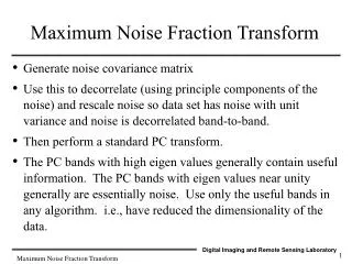
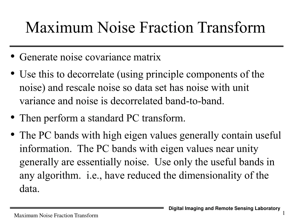
1. Maximum Noise Fraction Transform • Generate noise covariance matrix • Use this to decorrelate (using principle components of the noise) and rescale noise so data set has noise with unit variance and noise is decorrelated band-to-band. • Then perform a standard PC transform. • The PC bands with high eigen values generally contain useful information. The PC bands with eigen values near unity generally are essentially noise. Use only the useful bands in any algorithm. i.e., have reduced the dimensionality of the data. Maximum Noise Fraction Transform

2. This has an advantage over conventional processing in that PC selection is not dominated by noisy bands. • Useful in combination: looking at PC images and eigen values. Select those that carry spatially meaningful patterns and have significant variance. Maximum Noise Fraction Transform

3. Estimate noise statistics • This is easily done if a dark current image is available. If not, can take image data assume local constancy in scene and difference each pixel from one or more neighbors. This can be done full scene but works best in a uniform region. • Motivation: PC images don’t always show the common trend of less information and more noise as PC# increases. This is particularly the case with many band data. Maximum Noise Fraction Transform

4. Let is vector of image brightness values corresponding to image location x (x) is signal component of (x) is noise component of where S is covariance of signal (S(x)) N = covariance of noise (N(x)) and the S and N are assumed uncorrelated. If noise is multiplicative, can take logarithms and proceed. Maximum Noise Fraction Transform

5. Define the noise fraction to be • then the maximum noise fraction transform would choose the linear transform of the form • Y2 would be the band orthoganal to Y1 with the next largest noise function. • i.e., First MNF band has most noise, least info. • The last MNF band has the most info. Maximum Noise Fraction Transform

6. = ¢ Y ( x ) A Z ( x ) where é ù æ ö æ ö æ ö æ ö ç ÷ ç ÷ ç ÷ ç ÷ = A L ê ú ç ÷ ç ÷ ç ÷ ç ÷ è ø è ø è ø è ø ë û v v v v a a a a 1 2 3 n • The transform vectors are found to be the eigen vectors of N-1 • The eigen values µi are the noise fractions of the MNF bands Yi such that v v v v m The first eigen vect or a correspond s to , the largest eigen valu e 1 1 Maximum Noise Fraction Transform

7. Thus the last eigen value has highest S/N. • By eliminating first MNF bands or severely smoothing the noise in these bands we can improve image quality in back transform. Maximum Noise Fraction Transform

8. An alternative approach to achieving the same end • Note that this same effect is achieved if the standard PC transform is used on bands with uncorrelated noise with equal noise variance. • If is the transform that orthagonalizes the noise, i.e., such that is made up of the eigen vectors, of the noise covariance matrix and uni are the corresponding eigen values (i.e., the variance in the noise transform bands). Maximum Noise Fraction Transform

9. If we transform the image data Z(x) using the noise eigen vectors, i.e., and then normalize the Qi(x) values by then the noise variance in each of the normalized bands should be the same i.e., Maximum Noise Fraction Transform

10. where is transformed image (transformed using the eigen vectors of the noise covariance) normalized by the standard deviation of the noise in the transformed space, i.e., we have whitened the noise in the transform space between the Ri bands. We then compute the covariance matrix for the image data in the transform space, i.e., and transform the R(x) data into a new principal component space. The PC’s should now be ordered in a conventional fashion with the noise increasing with the PC rank. Maximum Noise Fraction Transform

11. However to take advantage of it we need to estimate the noise covariance N. • This is trivial if a dark field image is available, i.e., we assume any signal is noise and so the covariance of the dark field image is N. The noise can also be estimated if a region of the image that should have a constant digital count can be identified. Then if we subtract the mean DC of the region of interest (ROI) from all the pixels in the ROI, the covariance of the ROI after subtraction is an estimate of N. • In cases where these options are not available, we can assume localized uniformity in the signal data and simply assume the differences between adjacent pixels are an estimate of the noise. Maximum Noise Fraction Transform