1.3 Modeling with exponentially many constr.

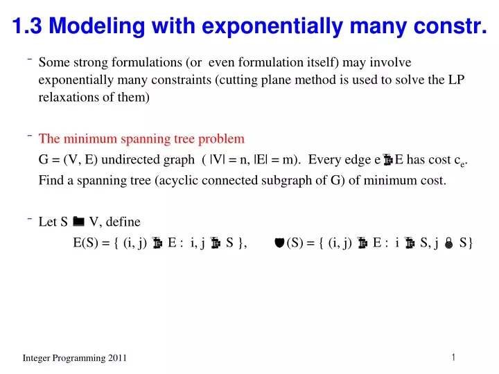
1. 1.3 Modeling with exponentially many constr. • Some strong formulations (or even formulation itself) may involve exponentially many constraints (cutting plane method is used to solve the LP relaxations of them) • The minimum spanning tree problem G = (V, E) undirected graph ( |V| = n, |E| = m). Every edge eE has cost ce. Find a spanning tree (acyclic connected subgraph of G) of minimum cost. • Let S  V, define E(S) = { (i, j)  E : i, j  S }, (S) = { (i, j)  E : i  S, j  S}

2. Subtour elimination formulation min  e  E ce xe  e  E xe = n-1,  e  E(S) xe  |S|-1, S  V, S  , V, xe  {0, 1} • Cutset formulation min  e  E ce xe  e  E xe = n-1,  e  (S) xe  1, S  V, S  , V, xe  {0, 1} • Thm 1.1 : (a) Psub  Pcut , and there exists examples for which the inclusion is strict. (b) Pcut can have fractional extreme points.

3. It can be shown that LP relaxation of subtour elimination formulation gives integer optimal solutions. (polymatroid) • Why consider IP formulation although there exist good algorithms (Kruskal, Prim)? • Algorithms may fail if problem structure changed a little bit: degree constrained spanning tree problem, Shortest total path length spanning tree problem, Steiner tree problem, capacitated spanning tree problem, … • Formulation of a basic problem may be used as part of a formulation for a larger complicated problem. • Theoretical analysis, e.g. strength of 1-tree relaxation of TSP.

4. The traveling salesman problem • G = (V, E) undirected graph. Every edge eE has cost ce. Find a tour (a cycle that visits all nodes) of minimum cost. • Cutset formulation minimize e  E ce xe subject to e   ({i}) xe = 2 , i  V e  (S) xe  2 , S  V, S  , V, xe  { 0, 1 }. • Subtour elimination formulation minimize e  E ce xe subject to e   ({i}) xe = 2 , i  V e  E(S) xe  |S| - 1 , S  V, S  , V, xe  { 0, 1 }. • LP relaxations of both formulations give the same solution set.

5. Remarks • For directed version of the problem, the following formulation is possible, which is smaller in size. But it is a bad formulation. (refer exercise 1.21 in text page 32) ui – uj + nyij n – 1 , ( i, j )  A, i, j  1, { i : ( i, j )  A} yij = 1 , j  V { j : ( i, j )  A} yij = 1 , i  V yij  { 0, 1 }, i, j  V • Note that, uj’s are continuous variables in the above formulation. • Undirected TSP is a special case of directed case, we may replace each edge by two directed arcs with opposite direction and having the same costs as the edge.

6. Is the formulation correct? The formulation has u, y variables. If (u*, y*) feasible, we only read y* values ( projection of (u*, y*) to y space) We need to show that (1) any tour solution y* satisfies the constraints and (2) any non-tour solution does not satisfy the constraints. (1) For any tour y*, if node i is k-th node in the tour, assign ui = k. (2) If y* is 0,1 and satisfies degree constraints, it is either a tour or consists of subtours. If subtours exist, there is one that does not include node 1. Add the constraints ui – uj + nyij n – 1 along the arcs in the subtour.

7. Comparing the LP relaxation of the cutset formulation (A) (in directed case version) and the LP relaxation of the previous formulation (B): It can be shown that the projection of the polyhedron B onto y space gives a polyhedron which completely contains A (the inclusion is strict), hence cutset formulation (or subtour elimination formulation) is stronger. • Although the previous formulation is not strong, it can be an alternative to use if you only have a generic IP software to use, not the sophisticated one to handle the cutset constraints.

8. How to Solve the LP relaxation of the Cut-Set Formulation? (many constr.) Solve LP relaxation (w/o cut-set constraints) If y* tour, stop. O/w find violated cut-set Solve LP after adding the Cut-set constraint.  violated cut-set? Y N Stop

9. If the obtained solution is not a tour, branch and apply the same procedure again. Choose the best solution • Branching : If yij* 0, 1, solve two subproblems after setting yij = 0, and yij =1. • Branch-and-cut approach ( cutting plane alg.) • Ideas for TSP formulation can be used for various routing, sequencing problems. • Branch-and-cut Ideas useful to solve many difficult IP problems. • What can we do for the LP with many variables? For the LP with many vars. and constraints? • TSP site: http://www.tsp.gatech.edu/

10. The perfect matching problem • Match n persons into pairs perfectly. Cost cij if person i is matched with person j. • minimize e  E ce xe subject to e   ({i}) xe = 1 , i  V xe  { 0, 1 }. • Pdegree  conv(F) (Fig 1.7) • Add e  (S) xe  1 , S  V, S  V, |S| odd or e  E(S) xe  (|S|-1)/2, S  V, S  V, |S| odd • Both have Pmatching = conv(F).

11. Cut covering problems • General problem class that includes many problems on network and graph G = (V, E), |V| = n, undirected graph f: 2V Z+ , D  V , costs ce 0 for e  E • Cut covering problems • minimize e  E ce xe subject to e   ({i}) xe = f({i}), i  D  V, e   (S) xe  f(S), S  V, xe  { 0, 1 }. • There exists an optimal solution which is minimal w.r.t. inclusion. (ce 0 )

12. minimize e  E ce xe subject to e   ({i}) xe = f({i}), i  D  V, e   (S) xe  f(S), S  V, xe  { 0, 1 }. • The minimum spanning tree D = , f(S) = 1, for all S  , V • The traveling salesman problem D = V, f(S) = 2, for all S  , V • The perfect matching problem D = V, f(S) = 1, for all S  , V with |S| odd • The Steiner tree problem T  V needs to be connected by a tree possibly using nodes in V \ T. D = , f(S) = 1, for all S with ST  , T = 0, otherwise

13. The survivable network design problem Costs ce , for all e  E, requirements rij for every pair of nodes i, j  V Select a set of edges from E at minimum cost, so that between every pair of nodes i and j there are at least rij paths that do not share any edges (rij edge-disjoint paths) D = , f(S) = maxiS, jV\S rij , S  , V • The vehicle routing problem

14. Dircted vs. undirected formulations • Steiner tree problem • minimize e  E ce xe subject to e   (S) xe  1,  S  V, S  T  , T, (1.8) xe  { 0, 1 }. • (a) Vi T  , i = 1, … , p. (b) Vi Vj = , i, j = 1, … , p, i  j. (c) i=1pVi = V Let (V1 , … , Vp ) be the set of edges, whose endpoints lie in different Vi . minimize e  E ce xe subject to e  ( V1, …, Vp) xe  p-1, (V1 , … , Vp ) satisfying (a)-(c) xe  { 0, 1 }. (1.9)

15. Directed version G=(V, E)  G=(V, A) ({i, j}  E  two arcs (i, j), (j, i)  A, cij = cji  0) Find a minimum cost directed subtree that contains a directed path between some given root vertex 1 (1  T), and every other terminal in T. minimize (i, j)  A cij yij subject to (i, j)+(S) yij  1,  S  V, 1S, T\S  , (1.10) yij + yji  1, e = {i, j}  E, yij  { 0, 1 }. can recover x by setting xe = yij + yji , for all e = {i, j}  E, • Zsteiner (T)  Zpartition (T)  ZDsteiner (T)

16. (1.8) is a special case of (1.9) with p = 2.  Zsteiner (T)  Zpartition (T) • Assume that the root vertex 1  V1 , and consider (i, j)+(V\Vk) yij  1, k = 2, … , p. Add above together with yji  0 for j  Vk , k = 2, … , p and i V1 , (i, j)E  e  ( V1, …, Vp) (yij + yji )  p-1. setting xe = yij + yji , we get feasible x for the linear relaxation of (1.9)  Zpartition(T)  ZDsteiner (T) There are examples such that Zsteiner (T) < ZDsteiner (T) • For TSP, directed formulation has the same strength

17. 1.4 Modeling with exponentially many variables • Column generation method Enumerate partial feasible solutions and represent their interactions in the master model. (Decomposition) Important modeling tool in applications • The cutting stock problem Large rolls of paper of width W (raw). Customer demand bi rolls of width wi (final), i = 1, … , m. ( wi W) Minimize the number of large rolls used while satisfying customer demand. • Cutting pattern j, (a1j , …, amj ) : produce aij rolls of width wi in jth cutting pattern (number of possible cutting patterns can be enormous) A feasible cutting pattern j must satisfy i=1m aij wi  W and aij is nonnegative integer. (integer knapsack constraint)

18. Formulation minimize j=1n xj subject to j=1n aij xj = bi , i = 1, … , m, xj  Z+ , j = 1, … , n • xj is the number of rolls of width W (raw) cut by cutting pattern j. • LP relaxation can be solved by column generation. Fractional optimal solution may be rounded down and a few more raws may be used to produce additional finals. (close to optimal)

19. Combinatorial auctions N: set of bidders, M: set of items being auctioned bj(S) : bid that bidder j is willing to pay for S  M Assume that if S  T = , bj(S) + bj(T)  bj(S  T) Bidders are allowed to bid on combinations of different items. Let b(S) = maxjN bj(S) • maximize SM b(S) xS subject to S: iS xS  1, i  M, xS  {0, 1}, S  M

20. The vehicle routing problem transportation network: G = (V, E), undirected, cost ce , e  E. Node 0 is central depot. Node i  V represents customers with demand di . Company has m vehicles with capacities qk , k = 1, … , m Assume demand of each customer cannot be divided into several vehicles. • Let xj = 1 if partial tour j is used, and zero, otherwise (j = 1, … , N) aij : equals one if node i is visited in partial solution j. cj : cost of tour j minimize c’x subject to Ax = e x  {0, 1}N