Download
1 / 40
400 likes | 405 Views
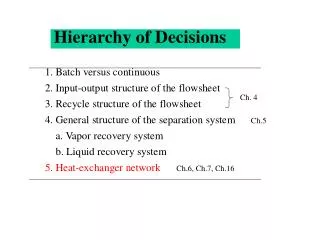
Hierarchy of Decisions. A DESIGN INSIGHT. HEN synthesis can be identified as a separate and distinct task in process design. I DENTIFY H EAT R ECOVERY AS A S EPARATE AND D ISTINCT T ASK IN P ROCESS D ESIGN. 9.60. 200 C. 18.2 bar. H1. 1.089. 36 C. 16 bar. RECYCLE.

E N D
A DESIGN INSIGHT HEN synthesis can be identified as a separate and distinct task in process design
IDENTIFY HEAT RECOVERYASA SEPARATEAND DISTINCT TASKIN PROCESS DESIGN. 9.60 200C 18.2 bar H1 1.089 36C 16 bar RECYCLE REACTION 7.841 126C 18.7 bar TO COLUMN D 201 C2 1.614 0 179 200C PURGE CW 180C 153C 35C FLASH 7 703 141C 40C 115.5C 17.3 bar 120C 17.6 bar FEED 5C 19.5 bar 114C C1 Flowsheet for “front end” of specialty chemicals process
200C Reactor 35C 200C RECYCLE TOPS Purge Reactor Product (H1) 35C 5C FEED (C1) PRODUCT (C2) 126C Heat exchange duties in specialty chemicals process: FOR EACH STREAM: TINITIAL, TFINAL, H = f(T).
= 1722 = 654 a ) DESIGN AS USUAL H 6 UNITS REACTOR C STEAM RECYCLE 70 1 。 。 STEAM 1652 3 2 654 COOLING WATER FEED PRODUCT
= 1068 = 0 b ) DESIGN WITH TARGETS H 4 UNITS REACTOR C STEAM 。 RECYCLE 1068 。 。 1 。 2 3 FEED PRODUCT
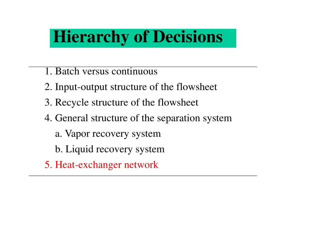
DESIGN PROCEDURE OF HEAT EXCHANGER NETWORKS Determine Targets. Energy Target - maximum recoverable energy Capital Targets minimum number of heat transfer units. minimum total heat transfer area Generate Alternatives to Achieve Those Targets. Modify the Alternatives Based on Practical Considerations. Equipment Design and Costing for Each Alternative. Select the Most Attractive Candidate.
ENERGY TARGETS (TWO-STREAM HEAT EXCHANGE) T Q =CP(TT-TS) TT TS H H
T (C) 200 UTILITY HEATING 140 135 115 100 70 UTILITY COOLING 350 300 400 H (KW) TWO-STREAM HEAT EXCHANGE IN THE T/H DIAGRAM
T (C) 200 UTILITY HEATING 130 135 T 120 100 70 UTILITY COOLING 350 300 400 H (KW) -100 +100 -100 =250 =400 =300 TWO-STREAM HEAT EXCHANGE IN THE T/H DIAGRAM
CONCLUSIONS ( ) ( ) 1. Total Utility Load Increa se Increa se 2. in = in Hot Utility Cold Utility
ENERGY TARGETS ( MULTIPLEHOT AND MULTIPLE COLD STREAMS) Construction of the Hot Composite Curve T T1 T2 T3 T4 T5 (T1-T2) (B) (T2-T3) (A+B+C) (T3-T4) (A+C) (T4-T5) (A) CP=B CP=A CP=C H
Construction of Hot Composite Curve T (1) (2) (3) (4) T1 T2 T3 T4 T5 H
PINCH POINT Minimum hot utility T “PINCH” minimum cold utility H Energy targets and “the Pinch” with Composite Curves
Generalized heat-exchange system m hot Streams Qin Heat Exchange System n cold Streams Qout - Qin = H Qout or
The “Problem Table” Algorithm ---Linnhoff and Flower, AIChE J. (1978) Stream No. CP TSTT andType(KW/C)(C)(C) (C) (C) (1) Cold 2 20 25 T6 135 140 T3 (2) Hot 3 170 165 T1 60 55 T5 (3) Cold 4 80 85 T4 140 145 T2 (4) Hot 1.5 150 145 (T2) 30 25 (T6) Tmin = 10C
Subsystem # CPHot - CPcold TK HK T1* = 165C T2* = 145C T3* = 140C T4* = 85C T5* = 55C T6* = 25C 2 1 20 3.0 60 2 5 0.5 2.5 3 55 -1.5 -82.5 4 30 2.5 75 5 30 -0.5 -15 4 3 1
from subsystem #2 90C hot streams 145C Heat Exchange Subsystem (3) . . . . . . . . . . . . . . . Cold streams 80C 135C To subsystem #4
T1* = 165C -------------------------- ( 0 )------ T2* = 145C --------------------------( 60 )-----( 80 ) T3* = 140C -------------------------( 62.5 )---( 82.5 ) T4* = 85C -------------------------( -20.0 )-----( 0 ) T5* = 55C --------------------------( 55.0 )----( 75 ) T6* = 25C --------------------------( 40.0 )---- FROM HOT UTILITY minimum hot utility 20 H1 = 60 H2 = 2.5 H3 = -82.5 Pinch H4 = 75 H5 = -15 minimum cold utility 60 TO COLD UTILITY
The Grand Composite Curve 80 60 40 20 0 -20 Q(KW) CU Qc,min “Pinch” HU Qh,min 20 40 60 80 100 120 140 160 180 T6* T5* T4* T3*T2* T1*
SIGNIFICANCE OF THE PINCH POINT 1. Do not transfer heat across the pinch 2. Do not use cold utility above 3. Do not use hot utility below
Q Qh Qh HU Qc,min CU Qh,min Tc Tp Th T Qh Qh,min Qc Qc,min
Q CU Qc,min Qh,min HU Tc Tp T1 Th T
Q Qc CU2 Qh HU Qc,min CU1 Qh,min Tc Tp Th T
Q Qh,min HU Qc,min CU Tc Tp T1 Th T
Q Qh,min HU2 Qc,min Q1 CU Q2 HU1 Tc Tp T1 Tp’ Th T
H=27MW H= -30MW FEED 2 140 PRODUCT2 230 REACTOR 2 200 80 H=32MW FEED 1 20 REACTOR 1 180 250 OFF GAS 40 H= -31.5MW 40 PRODUCT1 40 A simple flowsheet with two hot streams and two cold streams.
Heat Exchange Stream Data Heat Supply Target capacity temp. temp. H flow rate CP Stream Type TS (C) TT (C) (MW) (MW C-1) 1. Reactor 1 feed Cold 20 180 32.0 0.2 2. Reactor 1 product Hot 250 40 -31.5 0.15 3. Reactor 2 feed Cold 140 230 27.0 0.3 4. Reactor 2 product Hot 200 80 -30.0 0.25
(a) HOT UTILITY (b) HOT UTILITY 245C 0MW 7.5MW H= -1.5 H= -1.5 235C 1.5MW 9.0MW H= 6.0 H= 6.0 195C -4.5MW 3.0MW H= -1.0 H= -1.0 185C -3.5MW 4.0MW H= 4.0 H= 4.0 145C -7.5MW 0MW H= -14.0 H= -14.0 75C 6.5MW 14.0MW H= 2.0 H= 2.0 35C 4.5MW 12.0MW H= 2.0 H= 2.0 25C 2.5MW 10.0MW COLD UTILITY COLD UTILITY The heat-flow cascade.
The grand composite curve shows the utility requirements in both enthalpy and temperature terms.
(a) Process HP Stream Process Fuel Boiler Feedwater (Desuperheat) BOILER LP Stream Condensate T* HP Steam LP Steam pinch CW H Grand composite curve allows different utility mixes to be evaluated.
(b) Hot Oil Return Fuel FURNACE Process Hot Oil Flow T* Hot Oil pinch CW H Grand composite curve allows different utility mixes to be evaluated. .
T* Theoretical Flame Temperature T*O T*TFT T*STACK QHmin Flue Gas Air T*TFT Fuel T*STACK T*O Ambient Temperature Stack Loss ambient temp. QHmin H Fuel Furnace Model
Increasing the theoretical flame temperature by reducing excess air or combustion air preheat reduces the stack loss! T* T*’TFT T*TFT Flue Gas T*STACK T*O Stack Loss H
T* T*TFT T* T*TFT T*ACID DEW T*PINCH T*O T*ACID DEW T*PINCH T*O (a) Stack temperature limited by acid dew point (b) Stack temperature limited by process away from the pinch Furnace stack temperature can be limited by other factors than pinch temperature.
§ “PROBLEM TABLE” ALFORITHM SUBSYSTEM TM TC=T 0 (T0) 1 (T1) 2 (T2) TP Tmin Hh2Hc2 Hh1 Hc1
§ “PROBLEM TABLE” ALFORITHM ENTHALPY BALANCEOFSUBSYSTEM As T = T1 - T2 0
(a) TC 300 250 200 150 100 50 0 HP Steam LP Steam 0 5 10 15 H(MW) Figure 6.26 Alternative utility mixes for the process in Fig. 6.2.
(b) TC 300 250 200 150 100 50 0 Hot Oil 0 5 10 15 H(MW) Figure 6.26 Alternative utility mixes for the process in Fig. 6.2.
T* 1800 1750 Flue Gas 300 250 200 150 100 50 0 0 5 10 15 H(MW) Figure 6.30 Flue gas matched against the grand composite curve of the process in Fig. 6.2