Download
1 / 49
490 likes | 572 Views
The Design of Application Specific Integrated Circuits with High Level Synthesis Approaches. Shiann-Rong Kuang ( 鄺獻榮 ) Assistant Professor Dept. of Computer Science and Engineering National Sun Yat-Sen University. Outlines. Introduction Novel High Level Synthesis Approaches

E N D
The Design of Application Specific Integrated Circuits with High Level Synthesis Approaches Shiann-Rong Kuang (鄺獻榮) Assistant ProfessorDept. of Computer Science and EngineeringNational Sun Yat-Sen University
Outlines • Introduction • Novel High Level Synthesis Approaches • Integrated Data Path Synthesis Approach • Pipelined Control Path Synthesis Approach • Dynamic Pipelining Approach • ASICs design • Binary Arithmetic Coder • Low-Error Fixed-Width Multipliers • Fuzzy Color Corrector • Future Work
Introduction • High level synthesis • Behavioral description register transfer level description • Data path synthesis and control path synthesis FSM t1=a-b; t2=c+t1; t3=e-f; x=d-t2; y=t1+t3; e t2 y a t1 x e t3 d b f _ +
Integrated Data Path Synthesis Approach • Data Path Synthesis • module selection, scheduling, and allocation: highly interdependent • separately solve them the best designs may not be explored • Proposed Data Path Synthesis Approach • combine module selection, scheduling, and allocation • general module selection model • module types with different attributes (delay, area, …) • a mixed-vertex compatibility graph model • solve it globally using partial clique partitioning
a t1 x e t2 y c-step 0 -1 e t3 c t3 d d f f b e 1 +2 -1,-3 -4 +2 +5 2 -4 ADD_2 SUB_1 3 +5 4 -3 a t2 y b t1 x c-step 0 +2 +5 -1 -3 -4 -1 -4 1 SUB_3 ADD_1 SUB_2 2 +2 3 -3 4 +5 e a c b d f Clock cycle=100ns, Latency=5, and performance constraint=500ns -1 -4 t1 t3 +2 t2 +5 -3 y x
c-step c-step c-step 0 0 0 -1 -4 -1 -4 1 1 1 +5 +2 +2 +5 2 2 2 -3 -1 -3 3 3 3 +2 -4 4 4 4 +5 -3 • Find all feasible Assignments • MCG transformations Initial MCG A131 A130 A132 A141 A140 A442 A430 A433 A432 A431 A441 |V1|=30, |V2|=0 A440 A332 A334 A343 A342 A333 A211 A212 A213 A222 A221 A450 A511 A521 A522 A513 A514 A523 A512
instance 1 A140 A431 A433 A432 A430 A442 A441 A440 best Decision: A140, A333 A334 :new instance (subtractor) A343 A222 A212 A213 A450 A513 A523 A514 A522 A512 instance 1 A432 A433 A431 A430 best Decision: A343,1 (using the old subtractor instance) A140 , A343 A441 A442 A212 A440 A514 A513 A523 A450 A522 MCG after iteration 1 MCG after iteration 2
instance 2 instance 1 instance 1 instance 2 A450 A140 , A343 A450 A140 , A343 instance 3 |V1|=0, |V2|=3 A212 , A514 A212 A514 c t3 d f e a t2 y b t1 x c-step 0 +2 +5 -1 -3 -4 -1 -4 1 SUB_3 ADD_1 SUB_2 2 +2 3 -3 4 +5 Final MCG MCG after iteration 3
Integrated Data Path Synthesis Approach • Experiments and Results
OL i(t) OL OL i(t) i(t) i(t+1) SL SL SL SL SL SL’’ SL’ s(t) s(t) s(t) SRs SRs SRs (c) (a) (b) OL OL i(t) i(t) i(t) CRs PRs i(t+1) i(t+1) i(t+1) SRs’ pipelined circuit s(t) s(t) s(t) SRs SRs SRs (d) (e) (f) Pipelined Control Path Synthesis Approach • Main Idea of Pipelining Control Path
Pipelined Control Path Synthesis Approach • Proposed Control Path Synthesis Approach • A problem: may violatethe control dependency • Modify the original BSTG by inserting no operation states • Theorem A BSTG satisfies all control dependencies if the distance Dij of states in each produce-consume state pair <Si, Sj>c satisfies one of the following conditions: Condition 1: if Sj is not a branch state, then Dij k. Condition 2: if Sj is a branch state, then Dij2k-1. • Nij : the minimal number of NOOPs needed to insert between <Si, Sj>c Nij = 2k-Dij-1, if Sj is a branch state; Nij = k-Dij, otherwise. • Minimize the number of NOOPs using ILP formulation
S1 c1 >1 BSTG [>1,+1] c2 >2 S2 +1 >1 [>2,-2] c3 >3 -2 S3 >2 [>3,+3] +3 >3 c1 c1 S4 S7 [c3:+7] [c3:-9] +4 [+4] +7 -9 c2 c2 S6 -8 +5 -6 +10 S5 S8 [-6] [+5] [c3:-8] [c3:+10] +11 S9 [+11] S1 [>1,+1] S2 2 [>2,-2] 2 S3 [>3,+3] 2 c1 c1 S7 [c3:+7] [c3:-9] S4 [+4] 1 c2 c2 S6 S5 S8 [-6] [+5] [c3:-8] [c3:+10] 2 2 v1 v3 S9 [+11] 2 1 v2 v4 (a) i1 i2 v1 2 v3 2 1 2 v4 v2 (b) SCDFG
S1 S1 [>1,+1] [>1,+1] S2 S2 [>2,-2] [>2,-2] N1 N1 N2 N2 c1 c1 S3 S3 [>3,+3] N3 [>3,+3] N3 c1 c2 c1 c1 c1 c1 c2 S4 S4 N4 N4 [+4] [+4] c2 c2 S7 S7 [c3:+7] [c3:-9] S6 S5 S5 S6 [-6] [+5] [-6] [+5] S8 S8 [c3:-8] [c3:+10] S9 [+11] [+11] S9 pipelined circuit control registers PR3 PRk-1 PR1 PR2 [c3:+7] [c3:-9] CL2 CL3 CLk CL1 [c3:-8] [c3:+10] state registers
14 16 14 12 12 10 5_EWF 10 8 Cond2 8 6 6 5_EWF 4 4 Cond2 2 2 k k 0 0 0 2 4 6 8 10 12 0 2 4 6 8 10 12 lits 600 PRs 500 500 400 5_EWF 400 5_EWF Cond2 300 Cond2 300 200 200 100 k 100 k 0 2 4 6 8 10 12 0 0 2 4 6 8 10 12
Dynamic Pipelining Approach • Pipelining • In most of existing pipelining techniques, latency is fixed or has some fixed values • In some loops of ASICs, variant loop execution length and time-relative data dependencies between the different iterations make them to be pipelined inefficiently or impossibly • Dynamic pipelining • A new loop scheduling approach to pipeline the loop using variant latencies • Controller consists of two interactive finite state machines while(c1) { while(c2) { } }
iteration Latency=5 Latency=6 Latency=4 Phase 1 Phase 2 Phase 3 i i+1 i+2 i+3 i+4 time : the stages in which no operation is performed Dynamic Pipelining Approach
An Example of Dynamic Pipelining j=1; while (N>j) { /* N is the number of data which needs to be sorted */ i=j-1; temp=a[j]; while (temp<a[i] && i 0) { a[i+1]=a[i]; i=i-1; } a[i+1]=temp; j++; }
S1: j=1; ………......................…...………………....….…....o1 S1: j=1; ………......................…...………………....….…....o1 S2: O_loop: if(N j) goto End_O; …......…...……..o2 i=j-1; …….......................……………………….…........…o3 r_add=j; ………….….........…….………….…o4 S3: j++; ………….……..............…………………….........….o5 temp=a[r_add]; ……..….……………...……………..….o6 S4: I_loop: r_add=i; ……..…………….....……..….........o7 S5: data=a[r_add]; …………………..….........…..……......o8 S6: w_add=i+1; ………………………..…....…........…o9 if (!(temp<data && i 0)) goto End_I; ….o10 S7: a[w_add]=data; ………........…….……….......o11 i=i-1; gotoI_loop; …….......…………………o12 S8: End_I: a[w_add]=temp; gotoO_loop; ………........…o13 End_O:
Init S2 S1 S3 S8 Noopo Noopi S6 S5 S4 S7 start done [start=1] co [done=ci] done co done done start BSTGi Noopo S6,i start done S7,i PS1 S4,i S5,i [done=1] PS2 [done=ci] S5,i+1 Noopo S4,i+1 S6,i done done start S7,i start [done=1] [done=ci] S5,i+1 S4,i+1 done start • BSTG Partitioning BSTGo • Inner Loop Pipelining new PBSTGi original PBSTGi
S4 S5 Init S1 S2 S3 Noopi S8 done [start=1] co co done S2 S3 S4 S5 S2 S3 S4 S5 L=2 L=1 S2 S3 S4 S5 S2 S3 S4 S5 S2 S3 S4 S5 repeating pipeline body iteration i i+1 i+2 S2 S3 S4 S5 N1 S2 S3 S4 S5 N1 N2 N2 N3 N3 S8 S8 S2 S3 S4 S5 N1 N2 N3 S8 - i 1 S2 S3 S4 S5 N1 N2 N3 S8 • Outer Loop Pipelining new BSTGo : L=3 unwind the loop body four times
Noopx [start=1] co done done Noopi S5,i N1,i N2,i done S3 S8 S1 S2 S8 S4 Init done S2,i+1 S4,i+1 S3,i+1 co done [start=1] done repeating pipeline body Noopx co done PS1 [start=1] co done PS3 PS2 done S8,i N3,i N2,i+1 done S5,i+1 N1,i+1 S4,i+2 co done S3,i+2 S2,i+2 [start=1] co done done start PS1 PS2 Noopo done start S6,i S7,i [done=1] [done=ci] S5,i+1 S4,i+1 done start start final PBSTGo final PBSTGi
Datapath Allocation • Controller Architecture inner controller done ci Eq. (3.4) combinational logic Control signals from datapath to datapath state registers start co outer controller Mux combinational logic Eq. (3.3) state registers run Eq. (3.5)
- i 1 S S S S S S S S S S S S S S 2 3 4 5 6 7 4 5 6 7 4 5 6 8 S S S S S S 2 3 4 5 6 8 S S S S S S S S S S 2 3 4 5 6 7 4 5 6 8 An execution example iteration i S S S S S S S S S S S S S S S S S S 6 2 3 4 5 6 7 4 5 6 7 4 5 6 7 4 5 8 i +1 i +2 latency=5 latency=3 latency=3 latency=7 Nop PS1 PS2 PS1 PS1 PS2 PS1 PS2 PS1 PS1 PS2 PS1 PS2 PS1 PS2 PS1 PS1 Nop Nop PS1 PS2 PS1 inner PS1 outer PS1 PS2 PS3 PS1 PS2 PS3 PS1 Nop Nop PS2 PS3 PS1 Nop Nop Nop Nop PS2 PS3 PS1 PS2 PS3 PS1 PS2 S6 S4 S7 S5 S6 S4 S6 S4 S7 S5 S6 S4 S7 S5 S6 S4 S6 S4 S7 S5 S6 S4 S7 S5 S6 S4 S7 S5 S6 S4 S6 S4 S6 S4 S7 S5 S6 S4 state(i) S6 S4 N3 S5 S2 S8 N1 S3 N3 S5 S2 N3 S5 S2 S8 N1 S3 N3 S5 S2 N3 S5 S2 S8 N1 S3 N3 S5 S2 S8 N1 S3 S8 N1 S3 S8 N1 S3 state(o) N2 S4 N2 S4 N2 S4 N2 S4 N2 S4 done 1 0 0 1 0 0 0 0 1 0 0 0 0 0 0 1 1 1 1 0 0 1 0 start 1 0 0 1 0 0 1 1 1 0 0 1 1 1 1 1 0 0 1 0 0 1 0 run() 1 1 0 1 1 0 1 1 1 1 0 1 1 1 1 1 1 0 1 1 0 1 1
dynamic example data size sequential speedup pipelining Data1 10 56 31 1.81 Data2 10 236 121 1.95 Data3 10 108 57 1.89 Data4 10 112 59 1.90 Data5 100 596 301 1.98 Data6 100 20396 10201 2.00 Data7 100 9980 4993 2.00 Data8 100 10176 5091 2.00 Experimental Results • Comparing results of insertion sorter • Other examples
Binary Arithmetic Coder • Adaptive Binary Arithmetic Coder • Q-coder: compress mainly bilevel image data • a compression chip universal enough quickly compress any type of data that could still achieve a good compression ratio • proposed modified hardwared algorithm • a new probability estimation modeler using a table-look-up approach • a technique solves carry-over and source termination • fixed-width parallel multiplier • VLSI chip
Encoding Algorithm Encoding() { C=0x00; A=0xff; R=0x0000; S=0000000000; for (each input binary symbol) { phase1: Generate P('0'|S) by Eq. (4.5); phase2: AP=A* P('0'|S); if (input symbol=='0') A=AP; else { A=A-AP; C=C+AP; if (carry occurs) R++; } Update the adaptive modeler by Eq. (4.6); Shift the input symbol into S; phase3: while (MSB of A==0) normalization_of_encoding(); } Encode LPS and then output 17 consecutive '1'’s; }
En/De Adaptive Coder In_Data En_Input En_Input Input Shift_In 0 symbol De_Output S 1 Out_Data 1 De_Output En_Output 0 Output Asynchronous C’ symbol Input/Output P(‘0’|S) En/De Normalization Adaptive Arithmetic Path C Modeler Operation Unit Unit De_Input A handshaking A’ signals Control Path En_CL De_CL Init State registers En/De System Architecture
Low-Error Fixed-Width Multipliers • Fixed-Width Multiplier • multiplication operations used in many ASICs have the special fixed-width property • directly omit about half the adder cells of the conventional parallel multiplier a significant error would be introduced in the product • Low-Error Fixed-Width Multiplier • low-error fixed-width sign-magnitude multipliers • low-error fixed-width two’s complementmultipliers • reduced width multiplier (n < m < 2n)
ê ú ê ú ë û ê ê ë ú ú û Low-Error Fixed-Width Multipliers • Fixed-width sign-magnitude multipliers where Theorem: Given a , we have that and
x1 y0 x0y0 x3y0 x2y0 x4y0 x5 y0 Ha Ha Ha Ha Ha P0 x5y1 x0y1 x4y1 x3y1 x1y1 x2y1 P1 x5 y2 x4y2 x1y2 x0y2 x3y2 x2 y2 P2 x5y3 x1y3 x0y3 x3y3 x2y3 x4y3 x5 y0 P3 x5 y4 x1y4 x0y4 x3 y4 x2y4 x4y4 Fa Fa Fa Fa Fa Fa Fa Fa Fa Fa Fa Fa Fa Fa Fa Fa Fa Fa Fa Fa Fa Fa Fa Fa Fa Fa Fa Fa Fa Fa Fa Fa Fa Fa Fa Fa Fa Fa Fa cell AO: x4y1 AO1 x5y1 P4 x5y5 x4y5 x1 y5 x2y5 x0 y5 x3 y5 O1 C1 AO2 x3 y2 x5 y2 x4y2 P5 0 C2 O2 x2y3 AO3 x5y3 x3y3 x4y3 P11 P10 P9 P8 P7 P6 O3 C3 AO4 x1 y4 x5 y4 x3 y4 x2y4 x4y4 C4 O4 x0y5 AG x5y5 x4y5 x1 y5 x2y5 x3 y5 C5 Cg P11 P10 P9 P8 P7 P6 Ha X = x5 x4 x3 x2 x1 x0 Y = y5y4 y3y2y1y0 Sign-magnitude multiplier
x1 y0 x0y0 x3y0 x2y0 x4y0 x5 y0 Ha Ha Ha Ha Ha P0 P’ x5y1 x0y1 x4y1 x3y1 x1y1 x2y1 M P1 x5 y2 x4y2 x1y2 x0y2 x3y2 x2 y2 P2 x5y3 x1y3 x0y3 x3y3 x2y3 x4y3 P3 x5y0 x5 y4 x1y4 x0y4 x3 y4 x2y4 x4y4 Fa Fa Fa Fa Fa Fa Fa Fa Fa Fa Fa Fa Fa Fa Fa Fa Fa Fa Fa Fa Fa Fa Fa Fa Fa Fa Fa Fa Fa Fa Fa Fa Fa Fa Fa Fa Fa Fa Fa Fa x4y1 OR x5y1 P4 x5y5 x4y5 x3 y5 x2y5 x1 y5 x0 y5 x3y2 OR x5 y2 x4y2 P5 1 x2y3 OR x5y3 x3y3 x4y3 P11 P10 P9 P8 P7 P6 x1y4 OR x5 y4 x3 y4 x2y4 x4y4 x0y5 x5y5 x4y5 x3 y5 x2y5 x1 y5 cell OR: 1 P11 P10 P9 P8 P7 P6 Two’s complementmultiplier
x4y0 x5 y0 x1 y0 x0y0 x3y0 x2y0 x4y0 x5 y0 x3y1 AO x5y1 x4y1 P0 x5y1 x0y1 x4y1 x2 y2 x3y1 x1y1 x2y1 AO x5 y2 x4y2 x3y2 Ha Ha Ha Ha Ha Ha P1 x5 y2 x4y2 x1y3 x1y2 x0y2 x3y2 AO x2 y2 x5y3 x3y3 x2y3 x4y3 P’ M P2 x0y4 x5y3 x1y3 x0y3 x3y3 x2y3 x4y3 x5 y4 x1y4 x3 y4 x2y4 x4y4 Cg P3 x5 y4 x1y4 x0y4 x3 y4 x2y4 x4y4 x5y5 x4y5 x3 y5 x2y5 x1 y5 x0 y5 P4 x5y5 x4y5 x3 y5 x2y5 x1 y5 x0 y5 P5 1 P5 1 Fa Fa Fa Fa Fa Fa Fa Fa Fa Fa Fa Fa Fa Fa Fa Fa Fa Fa Fa Fa Fa Fa Fa Fa Fa Fa Fa Fa Fa Fa Fa Fa Fa Fa Fa Fa Fa Fa Fa Fa Fa Fa Fa Fa P11 P10 P9 P8 P7 P6 P11 P10 P9 P8 P7 P6 Reduced width multiplier
multipliers errors n =4 n =8 n =12 n =16 P' 48 1792 45056 983040 M M 32 1280 32768 720896 1 M 16 768 20480 458752 2 M 16 512 8192 196608 F M R two’s complement M 0.938 65.04 1570.32 30403.7 F M R (0.01) Â M 1 1 1 1 F e M 0.1 0.4 0.5 0.5 M R 16 256 4096 131072 P' 13.750 450.75 11267.75 245764.7 M M 5.375 187.89 3927.92 74497.4 1 e M 1.500 130.50 4099.50 98308.5 2 0.125 26.76 731.39 14629.6 P' 12.9 3.7 5.1 7.1 M M 5.6 2.5 2.3 2.8 1 M 1.6 1.9 2.5 3.2 2 Low-Error Fixed-Width Multipliers • Error comparison
Application (a) original (b) M1 (c) MF (d) MR1 (f) MS (e) MR2
(b) M1 (a) original
(c) MF (d) MR1
(f) MS (e) MR2
Fuzzy Color Corrector • Fuzzy Color Correction • in previous literature, the color correction process was modeled as a three-level fuzzy tree inference process • the algorithm in it is inefficient and its hardware implementation is then costly and slow • a new efficient fuzzy tree inference algorithm suitable for the center of gravity defuzzification method is proposed
modified fuzzy color correction algorithm Init: L=1; S1: while (input pattern Xi NULL) { S1: Calculate the address of rule memory (ROM); S2, S3: s1=ROM[address++]; D=s1; S4: k=0; PathL=0; d=ROM[address]; S5: while (k<8 && D>0) { S6: D=d;PathL=k;k++; } S5: if (1 k 7 &&|D| d/2) PathL=k; S7~S13: Calculate Xo using Eq. (6.6); S7: if (++L==4) L=1; }
2.5. Fuzzy Color Corrector • Proposed Sequential Architecture
dynamic file size pictures sequential speedup L pipelining (bytes) Pic1 148416 2704900 1370164 9.25 1.97 Pic2 230604 4345076 2193924 10.39 1.98 Pic3 974916 16898438 8139846 8.35 2.08 Pic4 1137198 20268056 10356836 9.11 1.96 Dynamic pipelined Design
Video Camera Display CPU Core Rate Control IP Video Enc. IP Video Dec. IP MEM VCI NNI NNI NNI NNI NNI External Networks Interconnection network NNI NNI NNI NNI NNI NNI O I R-FPGA other components Future Work System-on-a-Chip (SoC) Platform NNI: NoC Network Interface (ISO-OSI 7-Layer RM)
References [1] Jer-Min Jou, Shiann-Rong Kuang, Yeu-Horng Shiau, and Ren-Der Chen, “Design of A Dynamic Pipelined Architecture for Fuzzy Color Correction”, to be published in IEEE Transactions on VLSI Systems, 2002. [2] Jer-Min Jou, Yeu-Horng Shiau, Pei-Yin Chen, and Shiann-Rong Kuang, “A Low Cost Gray Prediction Search Chip for Motion Estimation”, Vol. 49, No. 7, pp. 928-938, July 2002. [3] Shiann-Rong Kuang, Jer-Min Jou, Ren-Der Chen, and Yeu-Horng Shiau, “Dynamic Pipeline Design of an Adaptive Binary Arithmetic Coder,” IEEE Transactions on Circuits & Systems Part II, Vol. 48, No. 9, pp. 813-825, September 2001. [4] Jer Min Jou, Shiann Rong Kuang, and Ren-Der Chen, “Design of Low-Error Fixed-Width Multipliers for DSP Applications,” IEEE Transactions on Circuits & Systems Part II, Vol. 46, No. 6, pp. 836-842, June 1999.
References [5] Jer-Min Jou, Shiann-Rong Kuang, and Ren-Der Chen, “A New Efficient Fuzzy Algorithm for Color Correction,” IEEE Transactions on Circuits & Systems Part I, Vol. 46, No. 6, pp. 773-775, June 1999. [6] Shiann-Rong Kuang, Jer-Min Jou, and Yuh-Lin Chen, “The Design of an Adaptive On-Line Binary Arithmetic Coding Chip,” IEEE Transactions on Circuits & Systems Part I, Vol. 45, No. 7, pp. 693-706, July 1998. [7] Jer-Min Jou and Shiann-Rong Kuang, “Design of a low-error fixed-width multiplier for DSP applications,” Electronics Letters, Vol. 33, No. 19, pp. 1597-1598, 1997. [8] Jer-Min Jou and Shiann-Rong Kuang, “A Library-Adaptively Integrated High Level Synthesis System,” Proceedings of NSC – Part A: Physical Science and Engineering, Vol. 19, No. 3, pp. 220-234, May 1995.