Download
1 / 12
120 likes | 234 Views
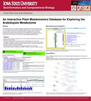
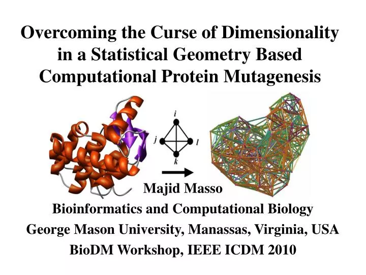
Overcoming the Curse of Dimensionality in a Statistical Geometry Based Computational Protein Mutagenesis. Majid Masso Bioinformatics and Computational Biology George Mason University, Manassas, Virginia, USA BioDM Workshop, IEEE ICDM 2010. center of mass (CM).

E N D
Overcoming the Curse of Dimensionality in a Statistical Geometry Based Computational Protein Mutagenesis Majid Masso Bioinformatics and Computational Biology George Mason University, Manassas, Virginia, USA BioDM Workshop, IEEE ICDM 2010
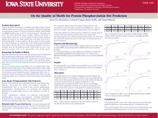
center of mass (CM) Abstract every amino acid residue to a point Atomic coordinates – Protein Data Bank (PDB) A22 L6 D3 F7 G62 K4 S64 R5 C63 Delaunay Tessellation of Protein Structure Aspartic Acid (Asp or D) Delaunay tessellation: 3D “tiling” of space into non-overlapping, irregular tetrahedral simplices. Each simplex objectively identifies a quadruplet of nearest-neighbor amino acids at its vertices.
Delaunay Tessellation of T4 Lysozyme • Ribbon diagram (left) based on PDB file 3lzm (164 residues) • Each amino acid residue represented as a CM point in 3D space • Tessellation of the 164 CM points (right) performed using a 12Å edge-length cutoff, for “true” residue quadruplet interactions
… 1bniA barnase 1jli IL-3 1rtjA HIV-1 RT 1efaB lac repressor Pool together all simplices from the tessellations, and compute observed frequencies of simplicial quadruplets Four-Body Statistical Potential Training set: 1,375 diverse high-resolution x-ray structures PDB Tessellate
Computational Mutagenesis: Residual Profiles ribbon CM trace 10 simplices share N163 vertex, and 10 total vertices; in the structure, N163 has 9 neighbors tessellation nonzero components identify the mutated position 163 and its 9 neighbors environmental change (EC)
Computational Mutagenesis: Residual Profiles • Nonzero ECs identify mutated position 163 and its 9 neighbors • So, the 19 mutants (N163A, N163C, etc.) at 163 will have nonzero ECs at the same 10 positions only, but nonzero values will differ • Each position has a different number of structural neighbors (min of 6, max of 19), which can be located throughout the sequence • Number of neighbors and their locations (position numbers) are dependent on the position being mutated
Experimental Data: Mutant T4 Lysozyme Activity • 2015 mutants synthesized by introducing the same 13 amino acids as replacements at 163 positions (all except the first) Rennell, D., Bouvier, S.E., Hardy, L.W. & Poteete, A.R. (1991) J. Mol. Biol.222, 67-88. • Each position yields either 12 or 13 mutants, depends on whether or not native amino acid there is also one of the 13 replacements • Mutant activity is based on plaque sizes on Petri dishes, 2 classes: “unaffected” = large plaques (same as native T4 lysozyme) “affected” = medium, small, or no plaques • 1377 “unaffected” and 638 “affected” T4 lysozyme mutants
Computational Mutagenesis: Feature Vectors • Approach 1 – represent mutants by 164D residual profile vectors; training set consists of all 2015 T4 lysozyme mutants • Approach 2 (dimensionality reduction) – select and order the 6 closest neighbors to the mutated position; create 7D vector of nonzero EC scores for mutated position and 6 closest neighbors • Approach 3 (subspace modeling) – segregate mutants by position number, consider each subset as a separate training set for classification, and combine the results; can be applied to 164D or 7D feature vectors
Supervised Classification • Algorithms: decision tree (DT), neural network (NN), support vector machine (SVM), and random forest (RF) • Testing: leave-one-out cross-validation (LOOCV) • Evaluation of performance: • Overall accuracy, or proportion of correct predictions: Q • Sensitivity and precision for both classes: S(U), P(U), S(A), and P(A) • Balanced error rate: BER • Matthew’s correlation coefficient: MCC
Results • Full training set with 164D surpasses 7D due to loss of implicit structural information (i.e., location of nonzeros in 164D vector) • Subspace modeling (SM) improves performance due to dramatic increase in S(A); 164D and 7D SM results are equal • SM with 164D vectors amounts to dimensionality reduction that uses the entire neighborhood of mutated position (unlike 7D, which uses only the 6 closest neighbors)
Conclusion and Future Directions • Residual profile vectors provide a natural way to introduce subspace modeling and achieve improved performance • Current work focused on inductive learning, future project could apply transductive learning to the dataset • Transduction allows us to also use vectors of all remaining mutants not classified experimentally – wet-lab collaborations can then validate our predictions • These techniques could be applied to a similarly comprehensive experimental dataset: 4041 mutants of lac repressor protein • Contact: mmasso@gmu.edu Slides available at: http://binf.gmu.edu/mmasso