Download
1 / 19
190 likes | 292 Views
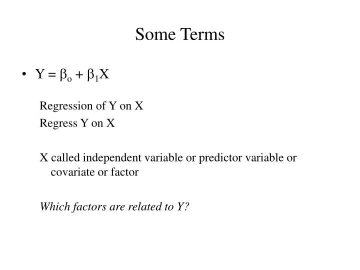
Some Terms. Y = b o + b 1 X Regression of Y on X Regress Y on X X called independent variable or predictor variable or covariate or factor Which factors are related to Y?. Multiple linear regression model. Y = b o + b 1 X 1 + b 2 X 2 + ... + b p X p + ε

E N D
Some Terms • Y = bo + b1X Regression of Y on X Regress Y on X X called independent variable or predictor variable or covariate or factor Which factors are related to Y?
Multiple linear regression model Y = bo + b1X1 + b2X2 + ... + bpXp + ε Y = outcome, dependent variable Xi = predictors, independent variables ε = error (or residual), normal; mean = 0, constant variance = 2 reflects how individuals deviate from others with the same values of x’s bi parameters describing the intercept and slope for each predictor
Evaluating Assumptions Y = bo + b1X1 • Y is normally distributed for each value of X • Can draw histogram overall for Y – can’t likely do for each X • Mean of Y changes linearly with X • Scatterplot of X and Y (see if points follow a line) • Plots of residuals versus X (or predicted values) • Variance s2 is constant for each X • Scatterplot of X and Y (see if deviations from line are same by X levels) • Remember there is no assumption on distribution of X
Plot of SBP Versus AGE PLOT sbp*age;
Plot of Model Residuals Versus AGE PLOTresidual.*age; Look for patterns. Patterns indicate relationship not linear. Note the sum of residuals = 0
Plot of Model Residuals Versus Predicted Values PLOTresidual.* predicted.; Look for patterns. For simple regression this is same as previous graph (residual versus x)
Evaluating Assumptions: Multiple Regression Y = bo + b1X1 + b2X2 • Y is normally distributed for each combination of Xs • Can draw histogram overall – can’t likely do for each X • Mean of Y changes linearly with each X and for every value of every other X • Variance s2 is constant for each combinations of X • Scatterplot of Y with each X (doesn’t really test assumption) • Scatterplot of residuals versus predicted values • Test for interactions
Interpreting Coefficients: Simple Regression Y = bo + b1X1 bo = mean of Y when X1 = 0 b1=change in mean of Y per 1-unit increase in X1 Suppose X1 = 5 Then Y = bo + 5b1 Suppose X1 = 6 Then Y = bo + 6b1 mean Yx1=6 – mean Yx1=5 = (b0 + 6b1) - (b0 + 5b1) = b1 Same difference for any x and x+1 chosen
Interpreting Coefficients: Multiple Regression Y = bo + b1X1 + b2X2 bo = mean of Y when X1 = 0 and X2 = 0 b1=change in mean of Y per 1-unit increase in X1for fixed X2 Suppose X1 = 5 Then Y = bo + 5b1 + X2b2 Suppose X1 = 6 Then Y = bo + 6b1 + X2b2 mean Yx1=6 – mean Y x1=5 = (b0 + 6b1 +X2b2) - (b0 + 5b1 +X2b2) = b1 Same value for every value of X2
Interpreting Relationships: Multiple Regression Y = bo + b1X1 + b2X2 b1 measures effect of X1 “adjusting for X2 ” or “above and beyond” X2 b2 measures effect of X2 “adjusting for X1” or “above and beyond” X1 If X1 is significantly related to Y in simple regression but not after including X2 in the model then: 1) The relationship of Y to X1 was confounded by X2 2) X1 is not an independent predictor of Y
Multiple Regression: R2 • Coefficient of Determination (R2) is proportion of variance explained by all variables in model • Adding variables to the model can only increase the R2. • Adding a highly correlated variable to a model will likely add little to R2. • Always interpret R2 in the context of the problem • Laboratory conditions yield high R2 • Real world yield lower R2 but X variables may still be important
Categorical Predictors; 0/1 coding Compare two groups; A and B. Let X = 0 for A, X = 1 for B Y = b0 + b1X For Group A, X= 0, mean outcome is; Y = b0 + b1(0) = b0 For Group B, X = 1, mean outcome is; Y = b0 + b1(1) = b0+ b1 mean Ygroup B - mean Ygroup A = (b0+ b1) - b0= b1 b0is the mean response for Group A b1is the difference in mean response between Group B and Group A
What if I use 1 and 2? Compare two groups; A and B. Let X = 1 for A, X = 2 for B Y = b0 + b1X For Group A, X= 5, mean outcome is; Y = b0 + b1(1) = b0 + b1 For Group B, X = 6, mean outcome is; Y = b0 + b1(2) = b0+ 2b1 mean Ygroup B - mean Ygroup A = (b0+ 2b1) – (b0 + b1 )= b1 b0 + b1 is the mean response for Group A b1is the difference in mean response between Group B and Group A
Categorical Predictors • More than two groups require more dummy (indicator) variables • Choose one group as reference group • Form a indicator variable for each of the other groups • K groups require K-1 indicator variables
Example - three groups Diet 1, 2, and 3; Choose “3” as reference group (could choose any of three) Y = b0 + b1X1 + b2X2 Diet 1: X1 = 1, X2 = 0 Diet 2: X1 = 0, X2 = 1 Diet 3: X1 = 0, X2 = 0 b0 is mean response for Diet 3 b1 is difference in mean response between Diet 1 and Diet 3 b2 is difference in mean response between Diet 2 and Diet 3
DUMMY CODING IN SAS * Assume variable diet with value 1-3; x1 = 0; x2 = 0; if diet = 1then x1 = 1; if diet = 2then x2 = 1; PROCREGDATA = lipid; MODEL chol = x1 x2; RUN;
DATA lipid; INFILE DATALINES; INPUT diet chol wt; * Assume variable diet with value 1-3; x1 = 0; x2 = 0; if diet = 1then x1 = 1; if diet = 2then x2 = 1; DATALINES; 1 175 140 1 180 135 1 185 145 1 190 140 1 195 155 2 190 140 2 195 135 2 200 150 2 205 155 2 210 150 3 180 140 3 185 150 3 190 155 3 195 145 3 200 150 ;
PROCMEANS NMEANSTD; CLASS diet; PROCREG; MODEL chol = x1 x2; RUN; PROC MEANS OUTPUT Analysis Variable : chol diet Obs N Mean Std Dev 1 5 5 185.0000000 7.9056942 2 5 5 200.0000000 7.9056942 3 5 5 190.0000000 7.9056942 PROC REG OUTPUT Parameter Estimates Parameter Standard Variable DF Estimate Error t Value Pr > |t| Intercept 1 190.00000 3.53553 53.74 <.0001 x1 1 -5.00000 5.00000 -1.00 0.3370 x2 1 10.00000 5.00000 2.00 0.0687
PROCREG; MODEL chol = x1 x2 ; MODEL chol = x1 x2 wt; RUN; PROC REG OUTPUT Parameter Standard Variable DF Estimate Error t Value Pr > |t| Intercept 1 190.00000 3.53553 53.74 <.0001 x1 1 -5.00000 5.00000 -1.00 0.3370 x2 1 10.00000 5.00000 2.00 0.0687 Parameter Standard Variable DF Estimate Error t Value Pr > |t| Intercept 1 84.28571 36.91070 2.28 0.0433 x1 1 -1.42857 4.13890 -0.35 0.7365 x2 1 11.42857 3.97892 2.87 0.0152 wt 1 0.71429 0.24868 2.87 0.0152