Statistical Data Analysis: Lecture 8

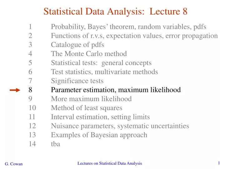
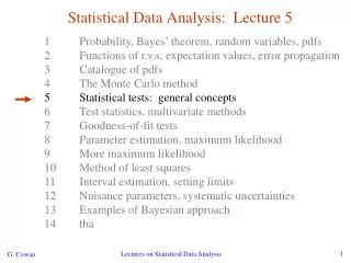
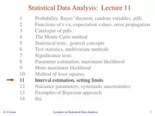
1. Statistical Data Analysis: Lecture 8 1 Probability, Bayes’ theorem, random variables, pdfs 2 Functions of r.v.s, expectation values, error propagation 3 Catalogue of pdfs 4 The Monte Carlo method 5 Statistical tests: general concepts 6 Test statistics, multivariate methods 7 Significance tests 8 Parameter estimation, maximum likelihood 9 More maximum likelihood 10 Method of least squares 11 Interval estimation, setting limits 12 Nuisance parameters, systematic uncertainties 13 Examples of Bayesian approach 14 tba Lectures on Statistical Data Analysis

2. Pre-lecture comments on problem sheet 7 Problem sheet 7 involves modifying some C++ programs to create a Fisher discriminant and neural network to separate two types of events (signal and background): Each event is characterized by 3 numbers: x, y and z. Each "event" (instance of x,y,z) corresponds to a "row" in an n-tuple. (here, a 3-tuple). In ROOT, n-tuples are stored in objects of the TTree class. Lectures on Statistical Data Analysis

3. Parameter estimation The parameters of a pdf are constants that characterize its shape, e.g. r.v. parameter Suppose we have a sample of observed values: We want to find some function of the data to estimate the parameter(s): ← estimator written with a hat Sometimes we say ‘estimator’ for the function of x1, ..., xn; ‘estimate’ for the value of the estimator with a particular data set. Lectures on Statistical Data Analysis

4. Properties of estimators If we were to repeat the entire measurement, the estimates from each would follow a pdf: best large variance biased We want small (or zero) bias (systematic error): → average of repeated measurements should tend to true value. And we want a small variance (statistical error): →small bias & variance arein general conflicting criteria Lectures on Statistical Data Analysis

5. An estimator for the mean (expectation value) Parameter: (‘sample mean’) Estimator: We find: Lectures on Statistical Data Analysis

6. An estimator for the variance Parameter: (‘sample variance’) Estimator: We find: (factor of n-1 makes this so) where Lectures on Statistical Data Analysis

7. The likelihood function Suppose the entire result of an experiment (set of measurements) is a collection of numbers x, and suppose the joint pdf for the data x is a function that depends on a set of parameters q: Now evaluate this function with the data obtained and regard it as a function of the parameter(s). This is the likelihood function: (x constant) Lectures on Statistical Data Analysis

8. The likelihood function for i.i.d.*. data * i.i.d. = independent and identically distributed Consider n independent observations of x: x1, ..., xn, where x follows f (x; q). The joint pdf for the whole data sample is: In this case the likelihood function is (xi constant) Lectures on Statistical Data Analysis

9. Maximum likelihood estimators If the hypothesized q is close to the true value, then we expect a high probability to get data like that which we actually found. So we define the maximum likelihood (ML) estimator(s) to be the parameter value(s) for which the likelihood is maximum. ML estimators not guaranteed to have any ‘optimal’ properties, (but in practice they’re very good). Lectures on Statistical Data Analysis

10. ML example: parameter of exponential pdf Consider exponential pdf, and suppose we have i.i.d. data, The likelihood function is The value of t for which L(t) is maximum also gives the maximum value of its logarithm (the log-likelihood function): Lectures on Statistical Data Analysis

11. ML example: parameter of exponential pdf (2) Find its maximum by setting → Monte Carlo test: generate 50 values using t = 1: We find the ML estimate: Lectures on Statistical Data Analysis

12. Functions of ML estimators Suppose we had written the exponential pdf as i.e., we use l = 1/t. What is the ML estimator for l? For a function a(q) of a parameter q, it doesn’t matter whether we express L as a function of a or q. The ML estimator of a function a(q) is simply So for the decay constant we have is biased, even though is unbiased. Caveat: Can show (bias →0 for n →∞) Lectures on Statistical Data Analysis

13. Example of ML: parameters of Gaussian pdf Consider independent x1, ..., xn, with xi ~ Gaussian (m,s2) The log-likelihood function is Lectures on Statistical Data Analysis

14. Example of ML: parameters of Gaussian pdf (2) Set derivatives with respect to m, s2 to zero and solve, We already know that the estimator for m is unbiased. But we find, however, so ML estimator for s2 has a bias, but b→0 for n→∞. Recall, however, that is an unbiased estimator for s2. Lectures on Statistical Data Analysis

15. Variance of estimators: Monte Carlo method Having estimated our parameter we now need to report its ‘statistical error’, i.e., how widely distributed would estimates be if we were to repeat the entire measurement many times. One way to do this would be to simulate the entire experiment many times with a Monte Carlo program (use ML estimate for MC). For exponential example, from sample variance of estimates we find: Note distribution of estimates is roughly Gaussian − (almost) always true for ML in large sample limit. Lectures on Statistical Data Analysis

16. Variance of estimators from information inequality The information inequality (RCF) sets a lower bound on the variance of any estimator (not only ML): Minimum Variance Bound (MVB) Often the bias b is small, and equality either holds exactly or is a good approximation (e.g. large data sample limit). Then, Estimate this using the 2nd derivative of ln L at its maximum: Lectures on Statistical Data Analysis

17. Variance of estimators: graphical method Expand ln L (q) about its maximum: First term is ln Lmax, second term is zero, for third term use information inequality (assume equality): i.e., → to get , change q away from until ln L decreases by 1/2. Lectures on Statistical Data Analysis

18. Example of variance by graphical method ML example with exponential: Not quite parabolic ln L since finite sample size (n = 50). Lectures on Statistical Data Analysis

19. Wrapping up lecture 8 We’ve seen some main ideas about parameter estimation: estimators, bias, variance, and introduced the likelihood function and ML estimators. Also we’ve seen some ways to determine the variance (statistical error) of estimators: Monte Carlo method Using the information inequality Graphical Method Next we will extend this to cover multiparameter problems, variable sample size, histogram-based data, ... Lectures on Statistical Data Analysis