Download
1 / 23
240 likes | 267 Views
Wringing a Table Dry: Using CSVZIP to Compress a Relation to its Entropy. Vijayshankar Raman & Garret Swart. Oxide is cheap, so why compress?. Make better use of memory Increase capacity of in memory database Increase effective cache size of on disk database Make better use of bandwidth

E N D
Wringing a Table Dry: Using CSVZIP to Compress a Relation to its Entropy Vijayshankar Raman & Garret Swart
Oxide is cheap, so why compress? • Make better use of memory • Increase capacity of in memory database • Increase effective cache size of on disk database • Make better use of bandwidth • I/O and memory bandwidth are expensive to scale • ALU operations are cheap and getting cheaper • Minimize storage and replication costs
Why compress relations? • Relations are important for structured information • Text, video, audio, image compression is more advanced than relational • Statistical and structural properties of the relation can be exploited to improve compression • Relational data have special access patterns • Don’t just “inflate.” Need to run selections, projections and aggregations
Our results • Near optimal compression of relational data • Exploits data skew, column correlations and lack of ordering • Theory: Compress m i.i.d. tuples to within 4.3 m bits of entropy (but theory doesn’t count dictionaries) • Practice: Between 8 and 40x compression • Scanning compressed relational data • Directly perform projections, equality and range selections, and joins on entropy compressed data • Cache efficient dictionary usage • Query short circuiting
Raw Data CSVZIP Flow Analyze • Analyze to determine compression plan • Compress to reduce size • Execute many queries over compressed data • Periodically update data and dictionaries ThisTalk Meta Data &Dictionaries Compress CompressedData Update Query NewRaw Data Results
Sources of Redundancy in Relations {“Apple”, “Pear”, “Mango”} in CHAR(10) • Column Value space much smaller than Domain • |C| << |domain(C)| • Type specific transformations, dictionaries • Skew in value frequency • H(C) << lg |C| • Entropy encoding (e.g. Huffman codes) • Column correlations within a tuple • H(C1, C2) << H(C1) + H(C2) • Column co-coding • Incidental tuple ordering • H({T1, T2, …, Tm}) ~ H(T1,T2, … , Tm) – m lg m • Sort and delta code • Tuple correlations • If correlated tuples share common columns, sort first on those columns 90% of fruits are “Apple” Mangos are mainly sold in August Mango buyers also buy paper towels
Male John 08/10/06 Mango Dict Dict Dict HuffmanEncode HuffmanEncode HuffmanEncode Input tuple Compression Process: Step 1 Male, John, 08/10/06, Mango Column 1 Column 2 Column 3 Co-codetransform Type specifictransform Sat 2006 w35 Column1 & 2 Column3.A Column3.B Male/John/Sat Male/John w35/Mango p = 1/512 p = 1/8 p = 1/512 ColumnCode ColumnCode ColumnCode 101101011 001 01011101 10110101100101011101 TupleCode
— — — Tuplecode Compression Process: Step 2 10110101110001011101 First tuple code 10110101110001011111 SortedTuplecodes 1 101101011100001100 1011010111000011101 PreviousTuplecode — 0000000000000000001 Delta 00000000000000000001 0000000000000000101 Dict HuffmanEncode 000 Delta Code 010 1110 Append CompressionBlock 10110101110001011101 101101011100010111010000101110 000 010 1110 Look Ma, no delimiters!
P1 – P6: Various projections of TPC-H tables P7: SAP SEOCOMPODF P8: TPC-E Customer Compression Results
Huffman Code Scan operations • SELECT SUM(price) FROM Sale WHERE week(saleDate) = 23 AND fruit = “Mango” AND year(saleDate) between 1997 AND 2005 • Scan this: 1011010110010101110101001 • Skip Over first column: Need length • Range Compare on 2nd column: year in 1997 to 2005 • Equality Compare 3rd column: Week = 23, fruit = Mango • Decode 4th column for aggregation • Segregated Coding: Faster operations, same compression • Assign Huffman Codes in order of length • |code(v)| < |code(w)| code(v) < code(w) • Sort codes within a length • |code(v)| = |code(w)| (v < w code(v) < code(w))
Segregated Coding: Computing Code Length • One code length Constant function • #define codeLen(w) 6 • Second largest code length << lg L1 cache size Use lookup table • #define codeLen(w) \ codeTable[x>>26] • Otherwise compare input with max code of each length • #define codeLen(w) \ (w <= 0b00111111…)?3 \ :(w <= 0b01001111…)?6 \ :(w <= 0b01010111…)?7 … )))
Segregated Coding: Range Query Value code switch (codeLen(w)) { case 3: return w>>28 != 0; 100 000 200 001 300 010 98 0110 case 4: return w >= 0b0111000000000000 && w <= 0b1000111111111111; 180 0111 220 1000 322 1001 87 10100 111 10101 190 10110 232 10111 case 5: return w >= 0b1011000000000000&& w <= 0b1101111111111111; } 256 11000 278 11001 298 11010 302 11011 SELECT * WHERE col BETWEEN 112 and 302 333 11100
Advantages of Segregated Coding • Find code length quickly • No access to dictionary • Fast Range query • No access to dictionary for constant ranges • Cache Locality • Because values are sorted by code length, commonly used values are clustered near the beginning of the array • The beginning of the array is most likely to be in cache, improving the cache hit ratio
Reuse predicates and values that depend on unchanged columns Sorting causes many unchanged columns Query Short Circuiting Previous Tuple: 101101011100001100 Delta Value: 0000000000000000101 Next Tuple: + 1011010111000011101 Common Bits: 1011010111000011 Unchanged Columns: Gender/FName Year Sex = MaleName = JohnYear ≥ 2005 Reusedpredicates: Reduces instructions but adds a branch!
Entropy Coding Shannon (1948), Huffman (1952) Arithmetic coding – Abramson (1963) Pasco, Rissanen (1976) Row or Page Coding Compress each row or page independently. Decompress on page load or row touch. Compression code is localized. [Oracle, DB2, IMS] Column-wise coding Each column value gets a fixed length code from a per column dictionary. [Sybase IQ, CStore, MonetDB] Pack multiple short values into 16 bit quantities and decode them as a unit to save CPU [Abadi/Madden/Ferreira] Delta coding Sort and difference or remove common prefix from adjacent codes [Inverted Indices, B-trees, CStore] Text coding “gzip” style coding using n-grams, Huffman codes, and sliding dictionaries [Ziv, Lempel, Welch, Katz] Order preserving codes Allows range queries at a cost in compression [Hu/Tucker, Antoshenkov/Murray/Lomet, Zandi/Iyer/Langdon] Lossy coding Model based lossy compression: SPARTAN, Vector quantization Selected Prior Work
Work in Progress • Analysis to find best: • Dictionaries that fit in L2 cache size • Set of columns to co-code • Column ordering for sort • Generate code for efficient queries on x86-64, Power5 and Cell • Don’t interpret meta-data at run time • Utilize architecture features • Update • Incremental update of dictionaries. Background merge of new rows. • Release of CSVZIP utilities
Observations • Entropy decoding uses less I/O, but more ALU ops than conventional decoding • Our technique removes the cache as a problem • Have to squeeze every ALU op: Trends in favor • Variable length codes makes vectorization and out-of-order execution hard • Exploit compression block parallelism instead • These techniques can be exploited in a column store
Entropy Encoding on a Column Store • Don’t build tuple code: Treat tuple as vector of column codes and sort lexicographically • Columns early in the sort: Run length encoded deltas • Columns in the middle of the sort: Entropy encoded deltas • Columns late in the sort: Concatenated column codes • Independently break columns into compression blocks • Make dictionaries bigger because only using one at a time
Entropy: A measure of information content • Entropy of a random variable R • The expected number of bits needed to represent the outcome of R • H(R) = ∑r domain(R) Pr(R = r) lg (1/ Pr(R = r)) • Conditional entropy of R given S • The expected number of bits needed to represent the outcome of R given we already know the outcome of S. • H(R | S) = ∑s domain(S)∑r domain(R) Pr(R = r & S = s) • lg (1/ Pr(R = r & S = s)) – H(S) • If R is a random relation of size n, then R is a multi-set of random variables {T1, …, Tn} where each random tuple Ti is a cross product of random attributes C1i … Cki
The Entropy of a Relation • We define a random relation R of size m over D as a random variable whose outcomes are multi-sets of size m where each element is chosen identically and independently from an arbitrary tuple distribution D. The results are dependent on H(D) and thus on the optimal encoding of tuples chosen from D. • If we do a good job of co-coding and Huffman coding, then the tuple codes are entropy coded: They are random bit strings whose length depends on the distribution of the column values but whose entropy is equal to their length • Lemma 2: The Entropy of random relation R of size m over a distribution D is at least m H(D) – lg m! • Theorem 3: The Algorithm presented compresses a random relation R of size m to within H(R) + 4.3 m bits, if m > 100
Proof of Lemma 2 • Let Rbe a random vector of m tuples i.i.d. over distribution D whose outcomes are sequences of m tuples, t1, …, tm. • Obviously H(R) is m H(D). • Consider an augmentation of R that adds an index to each tuple so that ti has the value i appended. Define R1 as a set consisting of exactly those values. H(R1) = m H(D) as there is a bijection between R1 andR • But the random multi-set R is a projection of the set R1 and there are exactly m! equal probability sets R1 that each project to each outcome of R so H(R1) ≤ H(R) + lg m! and thus H(R) ≥ m H(D) – lg m!
Proof sketch of Theorem 3 • Lemma 1 says: If R is random multi-set of m values over the uniform distribution 1..m and m > 100, then H(delta(sort(R))) < 2.67 m. • But we have values from an arbitrary distribution, so work by cases • For values longer than lg m bits, truncate, getting a uniform distribution in the range. • For values shorter than lg m bits, append random bits, also getting a uniform distribution.