Download
1 / 70
710 likes | 728 Views
Statistical tests for Quantitative variables (z-test, t-test & Correlation) BY Dr.Shaikh Shaffi Ahamed Ph.D., Associate Professor Dept. of Family & Community Medicine College of Medicine, King Saud University. Objectives:.

E N D
Statistical tests for Quantitative variables (z-test, t-test & Correlation) BY Dr.Shaikh Shaffi Ahamed Ph.D., Associate Professor Dept. of Family & Community Medicine College of Medicine, King Saud University
Objectives: • (1) Able to understand the factors to apply for the choice of statistical tests in analyzing the data . • (2) Able to apply appropriately Z-test, student’s t-test & Correlation • (3) Able to interpret the findings of the analysis using these three tests.
Choosing the appropriate Statistical test • Based on the three aspects of the data • Type of variables • Number of groups being compared & • Sample size
Statistical Tests Z-test: Study variable: Qualitative (Categorical) Outcome variable: Quantitative Comparison: (i)sample mean with population mean (ii)two sample means Sample size: larger in each group(>30) & standard deviation is known
Formulate H0 and H1 Select Appropriate Test Choose Level of Significance Calculate Test Statistic TSCAL (1)Determine Critical Value of Test Stat TSCR (3) Determine Prob Assoc with Test Stat (2) Determine if TSCR falls into (Non) Rejection Region (4) Compare with Level of Significance, Reject/Do not Reject H0 Draw Research Conclusion Steps for Hypothesis Testing
Example( Comparing Sample mean with Population mean): • The education department at a university has been accused of “grade inflation” in medical students with higher GPAs than students in general. • GPAs of all medical students should be compared with the GPAs of all other (non-medical) students. • There are 1000s of medical students, far too many to interview. • How can this be investigated without interviewing all medical students ?
What we know: • The average GPA for allstudents is 2.70. This value is a parameter. • To the right is the statistical information for a random sample of medical students: = 2.70
Questions to ask: • Is there a difference between the parameter (2.70) and the statistic (3.00)? • Could the observed difference have been caused by random chance? • Is the difference real (significant)?
The sample mean (3.00) is the same as the pop. mean (2.70). • The difference is trivial and caused by random chance. • The difference is real (significant). • Medical students are different from all other students.
Step 1: Make Assumptions and Meet Test Requirements • Random sampling • Hypothesis testing assumes samples were selected using random sampling. • In this case, the sample of 117 cases was randomly selected from all medical students. • Level of Measurement is Interval-Ratio • GPA is I-R so the mean is an appropriate statistic. • Sampling Distribution is normal in shape • This is a “large” sample (n≥100).
Step 2 State the Null Hypothesis • H0: μ = 2.7 (in other words, H0: = μ) • You can also state Ho: No difference between the sample mean and the population parameter • (In other words, the sample mean of 3.0 really the same as the population mean of 2.7 – the difference is not real but is due to chance.) • The sample of 117 comes from a population that has a GPA of 2.7. • The difference between 2.7 and 3.0 is trivial and caused by random chance.
Step 2 (cont.) State the Alternat Hypothesis • H1: μ≠2.7 (or, H0: ≠μ) • Or H1: There is a difference between the sample mean and the population parameter • The sample of 117 comes a population that does not have a GPA of 2.7. In reality, it comes from a different population. • The difference between 2.7 and 3.0 reflects an actual difference between medical students and other students. • Note that we are testing whether the population the sample comes from is from a different population or is the same as the general student population.
Step 3 Select Sampling Distribution and Establish the Critical Region • Sampling Distribution= Z • Alpha (α) = .05 • α is the indicator of “rare” events. • Any difference with a probability less than α is rare and will cause us to reject the H0.
Step 3 (cont.) Select Sampling Distribution and Establish the Critical Region • Critical Region begins at Z= ± 1.96 • This is the critical Z score associated with α= .05, two-tailed test. • If the obtained Z score falls in the Critical Region, or “the region of rejection,” then we would reject the H0.
When the Population σ is not known,use the following formula:
Test the Hypotheses • Substituting the values into the formula, we calculate a Z score of 4.62.
Two-tailed Hypothesis Test When α = .05, then .025 of the area is distributed on either side of the curve in area (C ) The .95 in the middle section represents no significant difference between the population and the sample mean. The cut-off between the middle section and +/- .025 is represented by a Z-value of +/- 1.96.
Step 5 Make a Decision and Interpret Results • The obtained Z score fell in the Critical Region, so we reject the H0. • If the H0 were true, a sample outcome of 3.00 would be unlikely. • Therefore, the H0 is false and must be rejected. • Medical students have a GPA that is significantly different from the non-medical students (Z = 4.62, p< 0.05).
Summary: • The GPA of medical students is significantly different from the GPA of non-medical students. • In hypothesis testing, we try to identify statistically significant differences that did not occur by random chance. • In this example, the difference between the parameter 2.70 and the statistic 3.00 was large and unlikely (p < .05) to have occurred by random chance.
Exercise Only: Diet Only: measure of variability = [(0.633)2 + (0.540)2] = 0.83 sample mean= 4.1 kg sample standard deviation = 3.7 kg sample size = n = 47 standard error = SEM2 = 3.7/ Ö47 = 0.540 sample mean= 5.9 kg sample standard deviation = 4.1 kg sample size = n = 42 standard error = SEM1 = 4.1/ Ö42 = 0.633 Comparison of two sample meansExample : Weight Loss for Diet vs Exercise Did dieters lose more fat than the exercisers?
Example : Weight Loss for Diet vs Exercise Null hypothesis:No difference in average fat lost in population for two methods. Population mean difference is zero. Step 1. Determine the null and alternative hypotheses. Alternative hypothesis:There is a difference in average fat lost in population for two methods. Population mean difference is not zero. Step 2. Sampling distribution: Normal distribution (z-test) Step 3. Assumptions of test statistic ( sample size > 30 in each group) Step 4. Collect and summarize data into a test statistic. The sample mean difference = 5.9 – 4.1 = 1.8 kg and the standard error of the difference is 0.83. So the test statistic: z = 1.8 – 0= 2.17 0.83
Example : Weight Loss for Diet vs Exercise Recall the alternative hypothesis was two-sided. p-value = 2 [proportion of bell-shaped curve above 2.17] Z-test table => proportion is about 2 0.015 = 0.03. Step 5. Determine the p-value. Step 6. Make a decision. The p-value of 0.03 is less than or equal to 0.05, so … • If really no difference between dieting and exercise as fat loss methods, would see such an extreme result only 3% of the time, or 3 times out of 100. • Prefer to believe truth does not lie with null hypothesis. We conclude that there is a statistically significant difference between average fat loss for the two methods.
Student’s t-test: Study variable: Qualitative ( Categorical) Outcome variable: Quantitative Comparison: (i)sample mean with population mean (ii)two means (independent samples) (iii)paired samples Sample size: each group <30 ( can be used even for large sample size)
Student’s t-test • Test for single mean • Whether the sample mean is equal to the predefined population mean ? • 2. Test for difference in means • Whether the CD4 level of patients taking treatment A is equal to CD4 level of patients taking treatment B ? • 3. Test for paired observation • Whether the treatment conferred any significant benefit ?
Steps for test for single mean • Questioned to be answered • Is the Mean weight of the sample of 20 rats is 24 mg? • N=20, =21.0 mg, sd=5.91 , =24.0 mg • 2. Null Hypothesis • The mean weight of rats is 24 mg. That is, The sample mean is equal to population mean. • 3. Test statistics --- t (n-1) df • 4. Comparison with theoretical value • if tab t (n-1) < cal t (n-1) reject Ho, • if tab t (n-1) > cal t (n-1) accept Ho, • 5. Inference
t –test for single mean • Test statistics n=20, =21.0 mg, sd=5.91 , =24.0 mg t = t .05, 19 = 2.093 Accept H0 if t < 2.093 Reject H0 if t >= 2.093 Inference : We reject Ho, and conclude that the data is not providing enough evidence, that the sample is taken from the population with mean weight of 24 gm
Lean 6.1 7.0 7.5 7.5 5.5 7.6 7.9 8.1 8.1 8.1 8.4 10.2 10.9 t-test for difference in means Given below are the 24 hrs total energy expenditure (MJ/day) in groups of lean and obese women. Examine whether the obese women’s mean energy expenditure is significantly higher ?. Obese 8.8 9.2 9.2 9.7 9.7 10.0 11.5 11.8 12.8
Null Hypothesis Obese women’s mean energy expenditure is equal to the lean women’s energy expenditure. Data Summary lean Obese N 13 9 8.10 10.30 S 1.38 1.25
Solution • H0: m1 - m2 = 0(m1 = m2) • H1: m1 - m2 ¹ 0 (m1¹ m2) • a = 0.05 • df = 13 + 9 - 2 = 20 • Critical Value(s): Reject H Reject H 0 0 .025 .025 t -2.086 0 2.086
Calculating the Test Statistic: Hypothesized Difference (usually zero when testing for equal means) • Compute the Test Statistic: _ _ ) ( ) ( - m - m - X X 1 2 1 2 t = n1 n2 df = n + n - 2 1 2 ( ) ( ) × 2 × 2 + n - 1 S n - 1 S 2 1 1 2 2 S = ( ) ( ) P n - 1 + n - 1 1 2
Developing the Pooled-Variance t Test • Calculate the Pooled Sample Variances as an Estimate of the Common Populations Variance: = Pooled-Variance = Size of Sample 1 = Variance of Sample 1 = Size of Sample 2 = Variance of sample 2
First, estimate the common variance as a weighted average of the two sample variances using the degrees of freedom as weights ( ) ( ) 2 2 n - 1 × S + n - 1 × S 1 1 2 2 2 S = ( ) ( ) P n - 1 + n - 1 1 2 ( ) ( ) 2 2 × . 13 - 1 × 38 + 9 - 1 1 . 25 1 . = 765 = 1 ) ( ) ( 13 - + 9 - 1 1
Calculating the Test Statistic: ( ) ) | | ( X X - - m - m - 10.3 - 0 8.1 1 2 1 2 = 3.82 t = = 2 1 + 13 1 9 S 1 . 76 P n n 1 2 tab t 9+13-2 =20 dff = t 0.05,20 =2.086
T-test for difference in means Inference : The cal t (3.82) is higher than tab t at 0.05, 20. ie 2.086 . This implies that there is a evidence that the mean energy expenditure in obese group is significantly (p<0.05) higher than that of lean group
Suppose we want to test the effectiveness of a program designed to increase scores on the quantitative section of the Graduate Record Exam (GRE). We test the program on a group of 8 students. Prior to entering the program, each student takes a practice quantitative GRE; after completing the program, each student takes another practice exam. Based on their performance, was the program effective? Example
Can represent each student with a single score: the difference (D) between the scores
Approach: test the effectiveness of program by testing significance of D Null hypothesis: There is no difference in the scores of before and after program Alternative hypothesis: program is effective → scores after program will be higher than scores before program → average D will be greater than zero H0: µD = 0 H1: µD > 0
Recall that for single samples: For related samples: where: and
Mean of D: Standard deviation of D: Standard error:
Under H0, µD = 0, so: From Table B.2: for α = 0.05, one-tailed, with df = 7, t critical = 1.895 2.714 > 1.895 → reject H0 The program is effective.
Z- value & t-Value “Z and t” are the measures of: How difficult is it to believe the null hypothesis? High z & t values Difficult to believe the null hypothesis - accept that there is a real difference. Low z & t values Easy to believe the null hypothesis - have not proved any difference.
Working with two variables (parameter) As Age BP As Height Weight As Age Cholesterol As duration of HIV CD4 CD8
A number called the correlation measures both the direction and strength of the linear relationship between two related sets of quantitative variables.
Correlation Contd…. • Types of correlation – • Positive – Variables move in the same direction • Examples: • Height and Weight • Age and BP
Correlation contd… • Negative Correlation • Variables move in opposite direction • Examples: • Duration of HIV/AIDS and CD4 CD8 • Price and Demand • Sales and advertisement expenditure