Download
1 / 48
480 likes | 545 Views
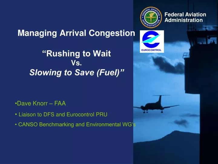
Managing Arrival Congestion “Rushing to Wait Vs. Slowing to Save (Fuel)”. Dave Knorr – FAA Liaison to DFS and Eurocontrol PRU CANSO Benchmarking and Environmental WG‘s. Outline. Part 1: Background and Motivation Part 2: Calculated Baseline Inefficiency

E N D
Managing Arrival Congestion “Rushing to Wait Vs. Slowing to Save (Fuel)” • Dave Knorr – FAA • Liaison to DFS and Eurocontrol PRU • CANSO Benchmarking and Environmental WG‘s
Outline • Part 1: Background and Motivation • Part 2: Calculated Baseline Inefficiency • Part 3: Estimating Terminal time and fuel savings from Speed reduction in Cruise Many Thanks to Co-authors: Philippe Enaud, Xing Chen, Marc Rose, Holger Hegendorfer and John Gulding
Motivation • Examples of Controlled Times of Arrival (CTA’s) to manage terminal area congestion: • ALOFT and MAESTRO Programs at Airservices Australia • Collaborative Flow Management – Airways NZ • NATS/United Trials into Heathrow • ATTILA with Delta into Atlanta • Morning Rush into Zurich • FAA ATTILA Trials at Charlotte • Tailored Arrivals into LAX and SFO • UPS use of ADS-B at Memphis • XMAN for FABEC…. And Lufthansa ASCAPE trials • Others?? • All cases motivated by fuel savings associated with incorporating FMS capabilities
Improvement Pools for Time and Fuel Savings Averages for Busiest 34 airports in the US and Europe *Under Review
Consider…. • In the US and Europe congestion management is applied based on projected arrival times …… but mainly implemented through ground holds
Consider…. Most flights receiving a ground delay will speed up (fly faster than cost index 0) after receiving a ground delay Premise for discussion: Once an arrival time constraint is established - FUEL is the only variable left for an airline to optimize (after safety)
Additional time within the last 100NM • Top 68 Busiest Airports average 3 min of delay and 120Kg additional fuel on approach
US and Europe - Establishing a Baseline • How much time and fuel is currently spent absorbing delay on approach? • Methodologies • Sample Airline data • Statistically based excess time using radar data, ac type and crossing times • Converting excess distance and level segments to time and fuel • Reduces impact of wind on estimates…
Taxi-In Efficiency • Efficiency • Efficiency • Efficiency • Taxi-Out • efficiency • 100NM • 40 NM • 100NM • Direction of • Flight • En-route • Flight • Notional Optimal • Route • efficiency • 2.5% • Actual Route • x • Arrival Fix • 40 nmi • Arrival • Airport • 100 nmi Inefficiency: Excess time in the last 100NM • Gate-to-Gate Originally Based on TAER Methodology – ATM2009 Updated to Better Account for Vertical Level-Offs – ATM2011
A100 Measure Jan 15, 2009 12:30-12:45pm 8 Arrivals in 15 Minutes 50 Flights Active within 15 Minutes 8.4 Minutes Average Inefficiency 40 nm 100 nm
Inefficiency Detected from RADAR Data Level Segments Vertical Inefficiency = ATC Constraints Direct Flight Horizontal Inefficiency Fuel (Act(x) – Fuel (Opt(x) Fuel (Opt(x) – Fuel (Opt(x0)
Change in Time Vertical Component hc – new altitude of level segment di – distance of level seg. Change in Fuel hi – altitude of level seg. From BADA v(h) – Speed at Alt h f(h) – Fuelburn at Alt h
- Cruise Altitude Nominal Fuel at Cruise Horizontal Component x - Actual Distance x0 - Minimum Distance From BADA Nominal Speed at Cruise v* benchmark speed from 100 nm to 40 nm for the group
Vertical Profile View SWA 1132 NWA 1176 SWA 186
Example Calculation SWA 186 • - 14 Min. “Delay” NWA 1176 SWA 1132 - 6 Min. “Delay” “Un-Impeded”
20091016 UAL870 Horizontal Calculation 100 to 40 excess distance: 0 40 to 0 excess distance: 0 Time improvement pool: 0 Fuel improvement pool: 0
Vertical Calculation Level distance: 0 Time saving pool: 0 Fuel saving pool: 0 • 20091016 UAL870
20090703 UAL870 Horizontal Calculation 100 to 40 excess distance: 0.42 nm 40 to 0 excess distance: 6.11 nm Time saving pool: 0.93 minute Fuel saving pool: 122.9 kg
Vertical Calculation Level distance: 19.1 nm Time pool saving: 1.7 minute Fuel saving pool: 160.7 kg 20090620 UAL870
Average Excess Time and Total Fuel by Facility 2009 ATL ORD JFK DFW 3.1 Minute Avg. Total Fuel a Product of Time, Fleet Mix and Total Volume of Operations
The CASE for Speed Control in Cruise • How much of the terminal area inefficiency can be recovered without changing throughput rates?? • Assumptions: • No speed adjustments for aircraft at the beginning of a “rush” • Used 1.5 to 5 minutes of absorbed delay as necessary for keeping pressure on the runways aircraft/ANSP flow control based speed • No fuel change estimated for slowing down in the cruise segment • Assumed 30, 60, 90 and 120 minute windows for absorbing time in cruise • If aircraft reaches cruise inside of 30 minutes left in cruise it is not considered in the pool
SAMPLE Impact of Mach Speed on Fuel Burn Maximum Range (MR) is “Cost Index 0” and minimizes fuel burn Long range cruise (LRC) is a compromise between speed and fuel Going slower in cruise burns less fuel ….up to a point! No fuel savings estimated for cruise speed reduction
Methodology for Minutes of Cruise Delay Absorption • Calculate time in cruise for each flight • Remove Climb (15min) and last 100nm • Establish variable for time available for speed reduction • Estimate potential time that can be absorbed for varying speed reductions • Example…5% reduction on a 90 minute cruise time implies up to 4.7 minutes can be absorbed (90/0.95-90) • Time absorbed in cruise is the difference between Potential time above and the Excess(previous slide) • Fuel Saved = Excess Fuel x time_saved/excess time
Challenges • Need better data on fuel saved by slowing in cruise • Implementation Issues remain with: • moving outside an Individual ANSP or Center’s sphere of influence • how to get times to pilots • how to enforce time windows (CTAs) • combining speed control with ground holds for shorter flights • how to handle equity and airline preferences for individual flights • conflict resolutions in cruise impact on achieving CTAs • controller roles and acceptance • Role of Simulations? • Additional Trials?
Conclusions • Potential pools for saving fuel thru speed changes can be estimated with basic ANSP data • Fuel savings can be achieved through speed control in cruise • Fuel can be saved both through slowing down and reducing excess time in the terminal area • Fuel Savings from speed control is achieved without increasing capacity or throughput • Worldwide implementation of CTA’s is growing and proving that fuel can be saved with speed adjustments today (without the benefit of full 4D trajectory management)
Fuel savings from speed control versus flight length (Europe 2009)
Vertical Profile View SWA 1132 NWA 1176 SWA 186
Example Calculation SWA 186 - 14 Min. “Delay” NWA 1176 SWA 1132 - 6 Min. “Delay” “Un-Impeded”
ANSP Quality of Service has 4 primary focus areas • Availability of Direct or Wind Optimal Routes • Maximizing Capacity and Throughput (Terminal and En Route) • Resilience of Capacity (IMC like VMC, time based separation for wind reduced capacity on final) 4. Managing necessary delay in the most fuel efficient manner (Measuring delay by phase of flight)
Calculating Potential Benefits from Reduced Speed in Cruise Example Methodology • Start with total excess terminal time on a per flight basis • Remove additional terminal time to keep pressure on runways (1.5, 2.5, & 5min) • Establish estimate for potential time absorption in cruise Additional Terminal Time into SFO Excess Minutes