Download

1 / 23
290 likes | 374 Views
Weighted k -set packing approximation. Speaker: Yoni Rozenshein Instructor: Prof. Zeev Nutov. Talk outline. Problem description and known approximations Interpretation in graphs (Independent Set Problem) The greedy local search method Approximation ratio Polynomial time implementation.

E N D
Weighted k-set packing approximation Speaker: Yoni Rozenshein Instructor: Prof. Zeev Nutov
Talk outline • Problem description and known approximations • Interpretation in graphs (Independent Set Problem) • The greedy local search method • Approximation ratio • Polynomial time implementation
Weighted k-set packing • Given a collection of weighted sets of size at most k,find a maximumweight collection of disjoint sets • Example with k = 3: Set packing Weight { 4, 5 } 16 { 2, 3, 5 } { 4 } 20 { 3, 4, 5 } 12 { 1, 5 } { 4 } 19
Hardness of the problem • For k = 2 we get the Maximum (Weighted) Matching Problem, which admits a polynomial time algorithm [Edmonds 1965] • The problem is NP-hard for k ≥ 3 [Karp 1972] • Reducible to k-SAT • k = 3: 3-Dimensional Matching
Approximation algorithms • OPT(I) – weight of the best solution (on instance I) • ALG(I) – weight of a given algorithm’s solution • Algorithm’s approximation ratioon instance I: • Algorithm’s approximation ratio: • We seek an algorithm that minimizes the ratio
The greedy algorithm • Repeatedly choose maximum-weight set S and delete from the family all sets that intersect S • Very fast; performance ratio k:
Local search heuristic • Replace a subset of the solution with a better subset • Repeat until “locally optimal” • How are the improvements chosen? • Polynomial running time? • Performance ratio k – 1 + ε [Arkin and Hassin 1997] • Can we improve on these ratios?
Interpretation in graphs • The sets’ intersection graph: • Nodes correspond to sets • Edges correspond to sets sharing elements • Set packing is a particular case of Maximum Weight Independent Set in intersection graphs • What characterizes intersection graphs arising from k-set packing instances? B A C E D
The characterization • The graph is k + 1-claw free • From now on, we consider the “Independent Set Problem in k + 1-claw free graphs” • Proof: • At most k elements in parent node • At least one in each child node • Pigeon-hole principle 1 Example with k = 3 2 k + 1-claw k + 1
Approach: Greedy local search • Previous algorithms combined • How are improvements chosen? • Polynomial running time? Greedy-Local-Search(G) I ← Greedy(G) while I is not locally optimaldo I’ ← local improvement of I I ← I’ end while output I
Local improvement scheme • Improvement: Pick some vϵI, add some of v’s neighbors, and delete any interfering nodes • The payoff factor is Pick B Add D Delete A, B B B B Local Improvement A A A Pick B C C C Add D Delete A, B E E E D D D
First algorithm: AnyImp • Polynomial running time? • For now, we will analyze the approximation ratio only AnyImp(G,α) I ← Greedy(G) while I is not locally optimaldo I’ ← any improvement of I with payoff factor ≥α I ← I’ end while output I
Analysis of the approximation ratio • Projection: “Distance” between I and OPT • proj(I) and w(I) maintain equilibrium minΦ(I) proj(I) w(I) Φ(I) ≈x⋅proj(I) + y⋅w(I)
Projection B B A A C C E E D D
Projection properties • Equilibrium property: • Local optimum property: • Result: (for any intermediate I) (for the final I) (for the final I)
Second algorithm: BestImp BestImp(G) I ← Greedy(G) while I is not locally optimaldo I’ ← an improvement of I with the highest payoff factor I ← I’ end while output I
Potential function In AnyImp’s potential*, d was constant • (Ii, di): Sub-sequence of local improvements Largest such that di (payoff factor) is descending: 2, 5, 3, 2, 4, 1.5, 3, 2, 1.2, 4, 3, 1.1 * I1 I2 I3 I4 (Final) (Greedy) I0 d1 = 2 d2 = 1.5 d3 = 1.2 d4 = 1.1
Potential properties • Equilibrium property: • Weight evaluation property: • Result: (for i=1, 2, …) (for i= 1, 2, …) (for the final I)
Running time analysis • Reminder: • Individual steps run in polynomial time • Number of improvements? Greedy-Local-Search(G) I ← Greedy(G) while I is not locally optimaldo I’ ← local improvement of I I ← I’ end while output I
Polynomial-time approximation scheme • Given an algorithm with approximation ratio ρ, produce a polynomial time algorithm with approximation ratio ρ + ε • Well-known example: Knapsack • The running time may depend strongly on ε (For example: Polynomial in 1/ ε) • Our greedy local search algorithm already runs in pseudo-polynomial time
PTAS: Weight scaling • Each improvement increases weight by 1 • Number of improvements at most:
Weight scaling – cont’d • Special case: • If we get within r of OPT'', we get within r(1 – ε) of OPT