Download

1 / 54
540 likes | 706 Views
Introduction to Linear M odelling Anne Segonds-Pichon v2019-03. Linear modelling is about language. Is there a difference between the 3 diets?. Can diet predict lobster weight ? Model(Diet) = Weight. Simple linear model. Linear regression

E N D
Linear modelling is about language Is there a difference between the 3 diets? Can diet predict lobster weight? Model(Diet) = Weight
Simple linear model • Linear regression • Correlation: is there an association between 2 variables? • Regression: is there an associationand • can one variable be used to predict the values of the other? Correlation = Association Regression = Prediction
Simple linear model • Linear regression models the dependence between 2 variables: • a dependenty and a independent x. • Causality • Model(x) = y • In R: • Correlation: cor() • Linear regression: lm() predictor response Model
Linear regression • Example:coniferlight.csv • conifer<-read.csv("coniferlight.csv") • Question: how is light (lux) affected by the depth (m) at which it is measured from the top of the canopy? • light = β0 + β1*depth plot(conifer$Light~conifer$Depth)
Linear regression • Linear modelling in R: lm(y~x) • Regression: lm(conifer$Light~conifer$Depth) • or: lm(Light~Depth, data=conifer) light = β0 + β1*depth light = 5014 - 292*depth
Linear regression linear.conifer<-lm(conifer$Light~conifer$Depth)
Linear regression abline() abline(a, b …) a=intercept, b=slope abline(linear.conifer) light = 5014 - 292*depth
Linear regression summary() lm(conifer$Light~conifer$Depth) summary(linear.conifer) p-value Coefficient of determination
Linear regression • Coefficient of determination: • R-squared (r2): • It quantifies the proportion of variance in Y that can be explained by X, it can be expressed as a percentage. • e.g. here 71.65% of the variability observed in light is explained by the depth at which it is measured in a conifer tree. • r: coefficient of correlation between x (depth) and y (light) • e.g. here: r = -0.846 so r2= -0.846 * -0.846 = 0.716 = R-squared cor(conifer)
Linear regression anova() summary(linear.conifer) Total amount of variability: 8738553 + 3457910 = 12196463 Proportion explained by depth: 8738553/12196463 = 0.716 anova(linear.conifer)
Linear regression the error Ɛ • Depth predicts about 72% (R-Squared) of the variability of light • so 28% is explained by other factors (e.g. Individual variability…) • Example: the model predicts 3627 lux at a depth of 4.75 m in a conifer. 3627 = 5014 - 292*4.75 y = β0 + β1*x + Ɛ 3627 lux 4.75m
linear.conifer<-lm(conifer$Light~conifer$Depth) Residual=error Ɛ light = 5014 - 292*depth 3627 = 5014 - 292*4.75 3627+1014=4641 light = 5014 - 292*depth+ Ɛ
Assumptions • The usual ones: normality, homogeneity of variance, linearity and independence. • Outliers: the observed value for the point is very different from that predicted by the regression model • Leverage points: A leverage point is defined as an observation that has a value of x that is far away from the mean of x • Influential observations: change the slope of the line. Thus, have a large influence on the fit of the model. One method to find influential points is to compare the fit of the model with and without each observation. • The Cook's distance statistic is a measure of the influence of each observation on the regression coefficients. • Bottom line: influential outliers are problematic.
Assumptions par(mfrow=c(2,2)) plot(linear.conifer) Linearity Normality Good model Homogeneity of variance Outliers Influential cases
Assumptions Linearity Normality Bad model Homogeneity of variance Outliers Influential cases
The linear model perspective Coyotes= Body length~Gender Protein = Expression~Cellline Goggles = Attractiveness~Alcohol and Gender
The linear model perspective Categorical predictor Continuous predictor • Coyotes body length • Is there a difference between the 2 genders? • becomes • Does gender predict coyote body length?
Example: coyotes • Questions: do male and female coyotes differ in size? • does gender predict coyote body length? • how much of body length is predicted by gender?
The linear model perspective Comparing 2 groups coyote<-read.csv("coyote.csv") remember to use tab! head(coyote) stripchart(coyote$length~coyote$gender, vertical=TRUE, method="jitter", las=1, ylab="Lengths", pch=16, col=c("darkorange","purple"), cex=1.5 ) length.means <- tapply(coyote$length, coyote$gender, mean) segments(1:2-0.15, length.means, 1:2+0.15, length.means, lwd=3 )
The linear model perspective Comparing 2 groups t.test(coyote$length~coyote$gender, var.equal=T) lm(coyote$length~coyote$gender) Females=89.71 cm, Males=89.71 + 2.34=92.05
The linear model perspective Comparing 2 groups lm(coyote$length~coyote$gender) Body length = β0 + β1*Gender Model Body length = 89.712 + 2.344*Gender
The linear model perspective Comparing 2 groups continuous y = β0 + β1*x conifer.csv light = 5014 - 292*depth categorical coyote.csv Body length = 89.712 + 2.344*Gender vector y = β0 + β1*x
The linear model perspective Comparing 2 groups Model Residuals
The linear model perspective Comparing 2 groups linear.coyote<-lm(coyote$length~coyote$gender) linear.coyote 86 coyotes Female 1: 89.71 + 3.29 = 93 cm
The linear model perspective Comparing 2 groups summary(linear.coyote) t.test(coyote$length~coyote$gender) anova(linear.coyote)
The linear model perspective Comparing 2 groups summary(linear.coyote) About 3% of the variability in body length is explained by gender. anova(linear.coyote) 118.1 + 3684.9 = 3803: total amount of variance in the data Proportion explained by gender: 118.1/3803 = 0.031
The linear model perspective Comparing 2 groups linear.coyote Assumptions par(mfrow=c(2,2)) plot(linear.coyote) Linearity Normality ~ shapiro.test() Equality of Variance leveneTest() Outliers
Example: coyote.csv One last thing • t.test(coyote$length~coyote$gender, var.equal = TRUE) • t.test(coyote.wide$female, coyote.wide$male, var.equal = TRUE) Long format Wide format
Example: coyote.csv • Questions: do male and female coyotes differ in size? • does gender predict body length? • Answer: Quite unlikely: p = 0.105 • how much of body length is predicted by gender? • Answer: About 3% (R2=0.031)
Exercises 10 and 11: coyotes and protein expressions • coyote.csv coyote<-read.csv("coyote.csv") • Run the t-test again t.test() • Run the same analysis using a linear model approach lm() • Compare the outputs and understand the coefficients from lm() • Use summary() and anova() to explore further the analysis • Work out R2 from the anova() output • Don’t forget to check the assumptions • protein.expression.csv protein<-read.csv("protein.expression.csv") • Prepare the file using melt()*,colnames()and na.omit() • Log-transformed the expression log10() • Run again the anova using aov() and summary() • Compare the 2 outputs • Use lm() and summary() for the linear model approach • Compare the outputs and understand the coefficients from lm() • Work out R2 from the anova() output • Don’t forget to check out the assumptions • *# reshape2 package #
Exercise 11: protein.expression.csv • Questions: is there a difference in protein expression between the 5 cell lines? • does cell line predict protein expression? • how much of the protein expression is predicted by the cell line?
Exercise 11: protein.expression.csv-Answers anova.log.protein<-aov(log10.expression~line,data=protein.stack.clean) summary(anova.log.protein) pairwise.t.test(protein.stack.clean$log10.expression,protein.stack.clean$line, p.adj = "bonf") TukeyHSD(anova.log.protein,"line")
Exercise 11: protein.expression.csv -Answers protein<-read.csv("protein expression.csv",header=T) ## more elegant way ## ## reshape2 package ## protein.stack.clean<-melt(protein, variable.name = "line", value.name = "expression", na.rm=TRUE) head(protein.stack.clean) stripchart(protein.stack.clean$expression~protein.stack.clean$line, vertical=TRUE, method="jitter", las=1, ylab="Protein Expression", pch=16, col=rainbow(5), log="y" ) expression.means<-tapply(protein.stack.clean$expression,protein.stack.clean$line,mean) segments(1:5-0.15,expression.means,1:5+0.15, expression.means, lwd=3) protein.stack.clean$log10.expression <- log10(protein.stack.clean$expression)
Exercise 11: protein.expression.csv -Answers linear.protein<-lm(log10.expression~line,data=protein.stack.clean) anova(linear.protein) summary(linear.protein) lm(log10.expression~line,data=protein.stack.clean)
Exercise 11:protein.expression.csv-Answers Model lm(log10.expression~line,data=protein.stack.clean) Expression= β0 + β1*Line Example: Line B = -0.03-0.25 = -0.28
Exercise 11: protein.expression.csv-Answers par(mfrow=c(2,2)) plot(linear.protein) Linearity Normality shapiro.test() Equality of Variance leveneTest() Outliers
Exercise 11: protein.expression.csv-Answers linear.protein<-lm(log10.expression~line,data=protein.stack.clean) summary(linear.protein) Proportion of variance explained by cell lines: 31% anova.log.protein<-aov(log10.expression~line,data=protein.stack.clean) summary(anova.log.protein) 2.691 + 6.046 = 8.737: total amount of variance in the data Proportion explained by gender: 2.691/8.737 = 0.308
Exercise 11: protein.expression.csv • Questions: is there a difference in protein expression between the 5 cell lines? • does cell line predict protein expression? • Answer: Yes p=1.78e-05 • how much of the protein expression is predicted by the cell line? • Answer: About 31% (R2=0.308)
Two-way Analysis of Variance Example: goggles.csv • The ‘beer-goggle’ effect • Study: effects of alcohol on mate selection in night-clubs. • Pool of independent judges scored the levels of attractiveness of the person that the participant was chatting up at the end of the evening. • Question: is subjective perception of physical attractiveness affected by alcohol consumption? • Attractiveness on a scale from 0 to 100 goggles<-read.csv("goggles.csv") head(goggles)
The linear model perspective Two factors fit.goggles<-aov(attractiveness~alcohol+gender+alcohol*gender,data=goggles) summary(fit.goggles) linear.goggles<-lm(attractiveness~alcohol+gender+alcohol*gender,data=goggles) anova(linear.goggles) (3332.3+168.7+1978.1)/(3332.3+168.7+1978.1+3487.5) = 0.611 R2 = 61% Model y = β0 + β1*x + β2*x2 + β3*x1x2
The linear model perspective Two factors linear.goggles<-lm(attractiveness~alcohol+gender+alcohol*gender,data=goggles) summary(linear.goggles) Attractiveness= β0 + β1Alcohol + β2Gender + β3Gender*Alcohol
Exercise 12: goggles.csv • goggles.csv goggles<-read.csv("goggles.csv") • Run again the 2-way ANOVA aov() • Run the same analysis using a linear model approach lm() • Work out R2 from the anova()output • Work out the equation of the model from the summary()output • Hint: Attractiveness= β0 + β1Gender + β2Alcohol + β3Gender*Alcohol • Predict the attractiveness of a date: • for a female with no drinks • for a male with no drinks • for a male with 4 pints
Exercise 12: goggles.csv-Answers • goggles.csv goggles<-read.csv("goggles.csv") • Predict the attractiveness of a date: • for a female with no drinks • 60.625+0+0 = 60.625 • for a male with no drinks • 60.625+0+6.250= 66.875 • for a male with 4 pints • 60.625-3.125+6.250-28.125= 35.625
The linear model perspective Categorical and continuous factors • Nothing special stats-wise with a mix of categorical and continuous factors • Same logic • But R makes it a little tricky to plot the model • treelight<-read.csv("treelight.csv") • plot(treelight$Light~treelight$Depth, col=treelight$Species, pch=16, cex=1.5) • legend("topright", c("Broadleaf", "Conifer"), pch=16, col=1:2)
The linear model perspective Categorical and continuous factors lm(Light~Depth*Species, data=treelight) linear.treelight<-lm(Light~Depth*Species, data=treelight) summary(linear.treelight) Complete model
The linear model perspective Categorical and continuous factors • Additive model: • linear.treelight.add<-lm(Light~Depth+Species, data=treelight) • summary(linear.treelight.add) No interaction abline() does not work directly here
The linear model perspective Categorical and continuous factors cf.add<-coefficients(linear.treelight.add) cf.add[1] It’s a vector! abline(cf.add [1], cf.add [2], col="black") abline(cf.add[1]+cf.add [3], cf.add [2], col="red") Broadleaf: Light = 7962.03 -262.17*Depth Conifer: Light = (7962.03-3113.03) -262.17*Depth
Exercise 13: treelight.csv • treelight.csv treelight<-read.csv("treelight.csv") • Plot the data • Run a linear model lm() • Extract the parameters from the additive model • Plot a line of best fit for each species • Extract the parameters from the complete model • Write the new equations for broadleaf and conifer species. • Plot a line of best fit for each species (use dashed lines to distinguish between • the 2 models). • Calculate the amount of light predicted: • In a conifer, 4 metres from the top of the canopy • In a broadleaf tree, 6 metres from the top of the canopy • How much of the variability of light is predicted by the depth and the species?
Exercise 13: treelight.csv cf<-coefficients(linear.treelight) plot(treelight$Light~treelight$Depth, col=treelight$Species, pch=16, las=1) legend("topright", c("Broadleaf", "Conifer"), pch=16, col=1:2) abline(cf[1]+cf[3], cf[2]+cf[4], col="red", lty="dashed") abline(cf[1], cf[2], col="black", lty="dashed") cf.add<-coefficients(linear.treelight.add) abline(cf.add [1], cf.add [2], col="black") abline(cf.add[1]+cf.add [3], cf.add [2], col="red")