Download
1 / 49
490 likes | 492 Views
This lecture provides an introduction to the concept of data in data mining, including data objects, attributes, and different types of attributes. It also covers discrete and continuous attributes, as well as various types of data sets. The lecture concludes with an overview of data preprocessing, including data cleaning and data reduction techniques.

E N D
Data Mining: Data Lecture Notes for Chapter 2 Introduction to Data Mining by Tan, Steinbach, Kumar
What is Data? • Collection of data objects and their attributes • An attribute is a property or characteristic of an object • Examples: eye color of a person, temperature, etc. • Attribute is also known as variable, field, characteristic, or feature • A collection of attributes describe an object • Object is also known as record, point, case, sample, entity, or instance Attributes Objects
Types of Attributes • There are different types of attributes • Nominal • Examples: ID numbers, eye color, zip codes • Ordinal • Examples: rankings (e.g., taste of potato chips on a scale from 1-10), grades, height in {tall, medium, short} • Interval • Examples: calendar dates, temperatures in Celsius or Fahrenheit. • Ratio • Examples: monetary, currency
Attribute Type Description Examples Operations Nominal The values of a nominal attribute are just different names, i.e., nominal attributes provide only enough information to distinguish one object from another. (=, ) zip codes, employee ID numbers, eye color, sex: {male, female} mode, entropy, correlation, 2 test Ordinal The values of an ordinal attribute provide enough information to order objects. (<, >) hardness of minerals, {good, better, best}, grades, street numbers median, percentiles, rank correlation Interval For interval attributes, the differences between values are meaningful, i.e., a unit of measurement exists. (+, - ) calendar dates, temperature in Celsius or Fahrenheit mean, standard deviation, Pearson's correlation, t and F tests Ratio For ratio variables, both differences and ratios are meaningful. (*, /) monetary quantities, electrical current geometric mean, harmonic mean, percent variation
Discrete and Continuous Attributes • Discrete Attribute • Has only a finite or countably infinite set of values • Examples: zip codes, counts, or the set of words in a collection of documents • Often represented as integer variables. • Note: binary attributes are a special case of discrete attributes • Continuous Attribute • Has real numbers as attribute values • Examples: temperature, height, or weight. • Practically, real values can only be measured and represented using a finite number of digits. • Continuous attributes are typically represented as floating-point variables.
Types of data sets • Record • Data Matrix • Document Data • Transaction Data • Graph • World Wide Web • Molecular Structures • Ordered • Spatial Data • Temporal Data • Sequential Data • Genetic Sequence Data
Record Data • Data that consists of a collection of records, each of which consists of a fixed set of attributes
Data Matrix • If data objects have the same fixed set of numeric attributes, then the data objects can be thought of as points in a multi-dimensional space. • Such data set can be represented by an m by n matrix, where there are m rows, one for each object, and n columns, one for each attribute
Document Data • Each document becomes a `term' vector, • each term is a component (attribute) of the vector, • the value of each component is the number of times the corresponding term occurs in the document.
Transaction Data • A special type of record data, where • each record (transaction) involves a set of items. • For example, consider a grocery store. The set of products purchased by a customer during one shopping trip constitute a transaction, while the individual products that were purchased are the items.
Graph Data • Examples: Generic graph and HTML Links
Chemical Data • Benzene Molecule: C6H6
Ordered Data • Sequences of transactions Items/Events An element of the sequence
Ordered Data • Genomic sequence data
Ordered Data • Genomic sequence data
Ordered Data • Spatio-Temporal Data Average Monthly Temperature of land and ocean
Why Preprocess the Data? • Measures for data quality: • Accuracy: correct or wrong, accurate or not • Completeness: not recorded, unavailable, … • Consistency: some modified but some not … • Believability: how trustable the data are correct? • Interpretability: how easily the data can be understood?
Major Tasks in Data Preprocessing • Data cleaning • Fill in missing values, smooth noisy data • Data Reduction • Sampling • Data Compression • Data transformation and data discretization • Normalization
Data Cleaning • Data in the Real World Is Dirty: Lots of potentially incorrect data, e.g., instrument faulty, human or computer error, transmission error • incomplete: lacking attribute values, lacking certain attributes of interest, or containing only aggregate data • e.g., Occupation = “ ” (missing data) • noisy: containing noise, errors, or outliers • e.g., Salary = “−10” (an error) • inconsistent: containing discrepancies in codes or names, e.g., • Age = “42”, Birthday = “03/07/2010” • Was rating “1, 2, 3”, now rating “A, B, C” • discrepancy between duplicate records • Intentional(e.g., disguised missing data) • Jan. 1 as everyone’s birthday?
How to Handle Missing Data? • Ignore the tuple: usually done when class label is missing (when doing classification)—not effective when the % of missing values per attribute varies considerably • Fill in the missing value manually: tedious + infeasible? • Fill in it automatically with • a global constant : e.g., “unknown”, a new class?! • the attribute mean • the attribute mean for all samples belonging to the same class: smarter
Noisy Data Noise: random error or variance in a measured variable Incorrect attribute values may be due to faulty data collection instruments data entry problems data transmission problems technology limitation 25
How to Handle Noisy Data? • Binning • first sort data and partition into (equal-frequency) bins • then one can smooth by bin means, smooth by bin boundaries, etc.
Binning Methods for Data Smoothing • Sorted data for price (in dollars): 4, 8, 9, 15, 21, 21, 24, 25, 26, 28, 29, 34 * Partition into equal-frequency (equi-depth) bins: - Bin 1: 4, 8, 9, 15 - Bin 2: 21, 21, 24, 25 - Bin 3: 26, 28, 29, 34 * Smoothing by bin means: - Bin 1: 9, 9, 9, 9 - Bin 2: 23, 23, 23, 23 - Bin 3: 29, 29, 29, 29 * Smoothing by bin boundaries: - Bin 1: 4, 4, 4, 15 - Bin 2: 21, 21, 25, 25 - Bin 3: 26, 26, 26, 34
Data Reduction: Sampling • Sampling: obtaining a small sample s to represent the whole data set N • Key principle: Choose a representative subset of the data • Simple random sampling may have very poor performance in the presence of skew • Develop adaptive sampling methods, e.g., stratified sampling:
Types of Sampling • Simple random sampling • There is an equal probability of selecting any particular item • Sampling without replacement • Once an object is selected, it is removed from the population • Sampling with replacement • A selected object is not removed from the population • Stratified sampling: • Partition the data set, and draw samples from each partition (proportionally, i.e., approximately the same percentage of the data) • Used in conjunction with skewed data
Raw Data Sampling: With or without Replacement SRSWOR (simple random sample without replacement) SRSWR
Sampling: Cluster or Stratified Sampling Cluster/Stratified Sample Raw Data
Sample Size 8000 points 2000 Points 500 Points
Data Reduction : Data Compression String compression There are extensive theories and well-tuned algorithms Typically lossless, but only limited manipulation is possible without expansion Audio/video compression Typically lossy compression, with progressive refinement Sometimes small fragments of signal can be reconstructed without reconstructing the whole
Data Compression Original Data Compressed Data lossless Original Data Approximated lossy
Data Transformation A function that maps the entire set of values of a given attribute to a new set of replacement values s.t. each old value can be identified with one of the new values Methods Smoothing: Remove noise from data Normalization: Scaled to fall within a smaller, specified range min-max normalization z-score normalization normalization by decimal scaling
Normalization • Min-max normalization: to [new_minA, new_maxA] • Ex. Let income range $12,000 to $98,000 normalized to [0.0, 1.0]. Then $73,000 is mapped to • Z-score normalization (μ: mean, σ: standard deviation): • Ex. Let μ = 54,000, σ = 16,000. Then • Normalization by decimal scaling Where j is the smallest integer such that Max(|ν’|) < 1
Similarity and Dissimilarity • Similarity • Numerical measure of how alike two data objects are. • Is higher when objects are more alike. • Often falls in the range [0,1] • Dissimilarity • Numerical measure of how different are two data objects • Lower when objects are more alike • Minimum dissimilarity is often 0 • Upper limit varies • Proximity refers to a similarity or dissimilarity
Euclidean Distance • Euclidean Distance Where n is the number of dimensions (attributes) and pk and qk are, respectively, the kth attributes (components) or data objects p and q.
Euclidean Distance Distance Matrix
Minkowski Distance • Minkowski Distance is a generalization of Euclidean Distance Where r is a parameter, n is the number of dimensions (attributes) and pk and qk are, respectively, the kth attributes (components) or data objects p and q.
Minkowski Distance: Examples • r = 1. City block (Manhattan, taxicab, L1 norm) distance. • A common example of this is the Hamming distance, which is just the number of bits that are different between two binary vectors • r = 2. Euclidean distance
Minkowski Distance Manhattan Distance Matrix Euclidean Distance Matrix
Common Properties of a Distance • Distances, such as the Euclidean distance, have some well known properties. • d(p, q) 0 for all p and q and d(p, q) = 0 only if p= q. (Positive definiteness) • d(p, q) = d(q, p) for all p and q. (Symmetry) • d(p, r) d(p, q) + d(q, r) for all points p, q, and r. (Triangle Inequality) where d(p, q) is the distance (dissimilarity) between points (data objects), p and q. • A distance that satisfies these properties is a metric
Similarity Between Binary Vectors • Common situation is that objects, i and j, have only binary attributes
Cosine Similarity • If d1 and d2 are two document vectors, then cos( d1, d2 ) = (d1d2) / ||d1|| ||d2|| , where indicates vector dot product and || d || is the length of vector d. • Example: d1= 3 2 0 5 0 0 0 2 0 0 d2 = 1 0 0 0 0 0 0 1 0 2 d1d2= 3*1 + 2*0 + 0*0 + 5*0 + 0*0 + 0*0 + 0*0 + 2*1 + 0*0 + 0*2 = 5 ||d1|| = (3*3+2*2+0*0+5*5+0*0+0*0+0*0+2*2+0*0+0*0)0.5 = (42) 0.5 = 6.481 ||d2|| = (1*1+0*0+0*0+0*0+0*0+0*0+0*0+1*1+0*0+2*2)0.5= (6) 0.5 = 2.245 cos( d1, d2 ) = .3150
Correlation • Correlation measures the linear relationship between objects
Visually Evaluating Correlation Scatter plots showing the similarity from –1 to 1.